Multivariate outliers
The function acc_multivariate_outlier uses the same
rules as acc_robust_univariate_outlier
for the identification of outliers. In the following example, we examine
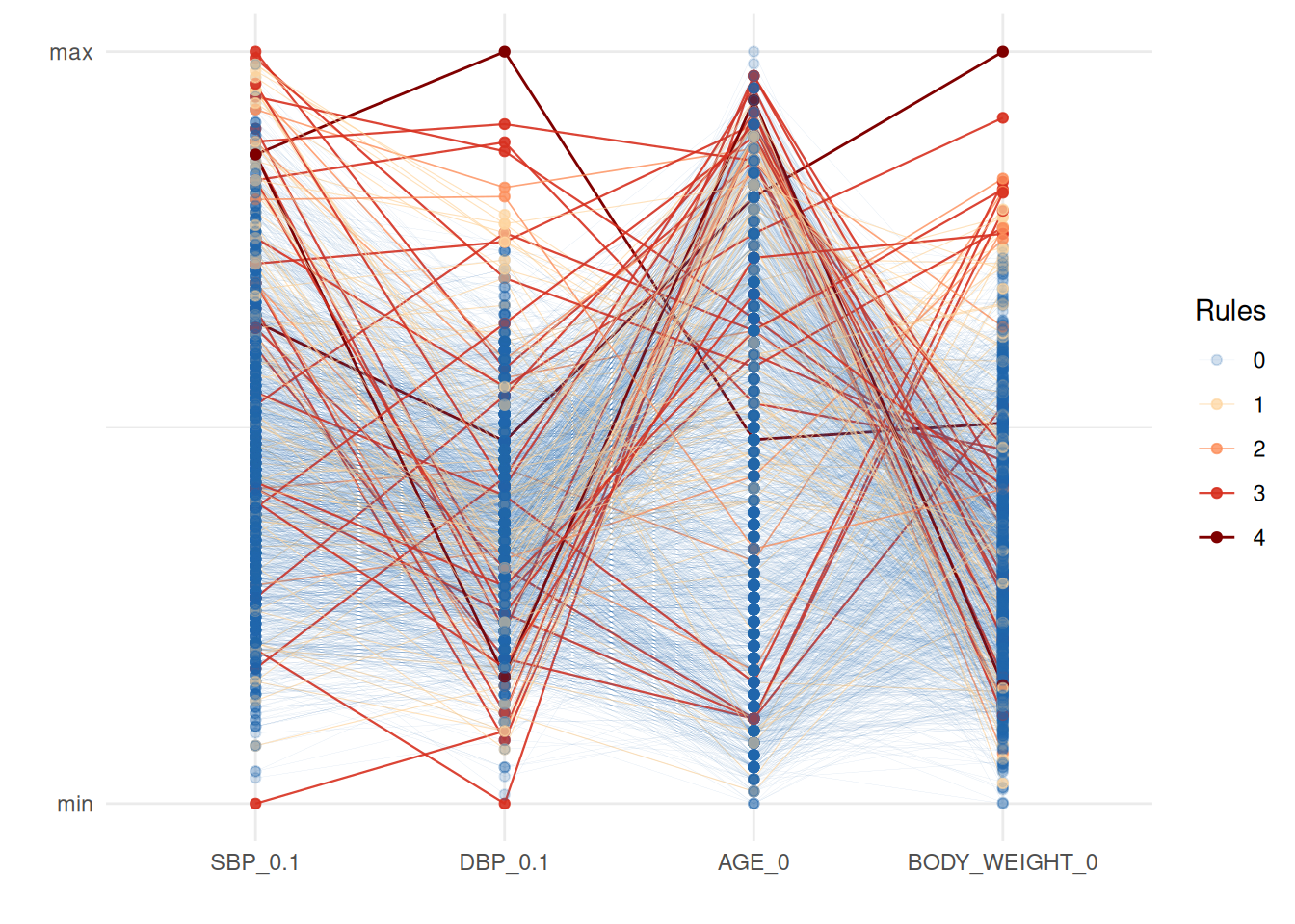
systolic and diastolic blood pressure measurements in relation to age
and weight, and a table output is created:
# Load dataquieR
library(dataquieR)

# Load data
sd1 <- prep_get_data_frame("ship")

# Load metadata
prep_load_workbook_like_file("ship_meta_v2")
meta_data_item <- prep_get_data_frame("item_level") # item_level is a sheet in ship_meta_v2.xlsx

# Apply indicator function
MVO_SBP0.1 <- acc_multivariate_outlier(
  variable_group = c("SBP_0.1", "DBP_0.1", "AGE_0", "BODY_WEIGHT_0"),
  study_data = sd1,
  meta_data = meta_data_item,
  id_vars = "ID",
  label_col = "LABEL"
)MVO_SBP0.1$SummaryTable| Variables | Tukey (N) | 3SD (N) | Hubert (N) | Sigma-gap (N) | NUM_acc_ud_outlm | PCT_acc_ud_outlm | GRADING |
|---|---|---|---|---|---|---|---|
| SBP_0.1 | DBP_0.1 | AGE_0 | BODY_WEIGHT_0 | 108 | 37 | 46 | 3 | 3 | 0.14 | 1 |
The number of outliers varies considerably depending on the criterion. Subsequently a parallel-coordinate-plot may be requested to further inspect results:
MVO_SBP0.1$SummaryPlot
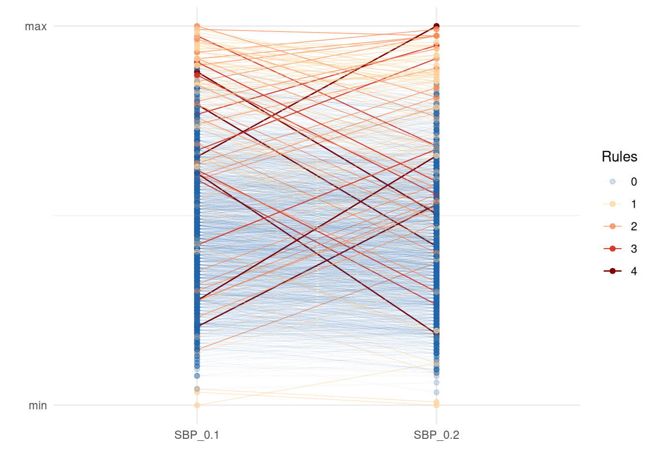
Another example is the inspection of the first and second systolic blood pressure measurements:
MVO_DBP <- acc_multivariate_outlier(
  variable_group = c("SBP_0.1", "SBP_0.2"),
  study_data = sd1,
  meta_data = meta_data_item,
  label_col = "LABEL"
)MVO_DBP$SummaryTable| Variables | Tukey (N) | 3SD (N) | Hubert (N) | Sigma-gap (N) | NUM_acc_ud_outlm | PCT_acc_ud_outlm | GRADING |
|---|---|---|---|---|---|---|---|
| SBP_0.1 | SBP_0.2 | 128 | 39 | 14 | 6 | 6 | 0.28 | 1 |
MVO_DBP$SummaryPlot


