Data Quality
Uncertain or Inadmissible numerical or time-date values
Both Uncertain numerical values
and Inadmissible numerical values, as
well as Uncertain time-date values
and Inadmissible time-date values,
can be calculated using con_limit_deviations).
When specifying limits = "SOFT_LIMITS" the check does not
identify inadmissible but uncertain values, according to the specified
ranges. An example call is:
# Load dataquieR
library(dataquieR)

# Load data
sd1 <- prep_get_data_frame("ship")

# Load metadata
prep_load_workbook_like_file("ship_meta_v2")
meta_data_item <- prep_get_data_frame("item_level") # item_level is a sheet in ship_meta_v2.xlsx

# Apply indicator function
MyValueLimits <- con_limit_deviations(
  study_data = sd1,
  meta_data  = meta_data_item,
  label_col  = "LABEL",
  limits     = "HARD_LIMITS"
)
A table output provides the number and percentage of all the range violations for the variables specifying limits in the metadata:
MyValueLimits$SummaryData| Variables | Limits | Below limits N (%) | Within limits N (%) | Above limits N (%) | All outside limits N (%) | |
|---|---|---|---|---|---|---|
| 1 | DBP_0.2 | HARD_LIMITS | 0 (0) | 2148 (100) | 0 (0) | 0 (0) |
| 5 | DBP_0.2 | DETECTION_LIMITS | 0 (0) | 2148 (100) | 0 (0) | 0 (0) |
| 9 | DBP_0.2 | SOFT_LIMITS | 4 (0.19) | 2134 (99.35) | 10 (0.47) | 14 (0.65) |
| 13 | BODY_HEIGHT_0 | HARD_LIMITS | 0 (0) | 2151 (100) | 0 (0) | 0 (0) |
| 17 | BODY_WEIGHT_0 | HARD_LIMITS | 0 (0) | 2150 (100) | 0 (0) | 0 (0) |
| 21 | WAIST_CIRC_0 | HARD_LIMITS | 0 (0) | 2148 (100) | 0 (0) | 0 (0) |
| 25 | EXAM_DT_0 | HARD_LIMITS | 0 (0) | 2154 (100) | 0 (0) | 0 (0) |
| 29 | CHOLES_HDL_0 | HARD_LIMITS | 0 (0) | 2138 (100) | 0 (0) | 0 (0) |
| 33 | CHOLES_LDL_0 | HARD_LIMITS | 0 (0) | 2126 (100) | 0 (0) | 0 (0) |
| 37 | CHOLES_ALL_0 | HARD_LIMITS | 0 (0) | 2139 (100) | 0 (0) | 0 (0) |
| 41 | AGE_0 | HARD_LIMITS | 1 (0.05) | 2153 (99.95) | 0 (0) | 1 (0.05) |
| 45 | SBP_0.1 | HARD_LIMITS | 0 (0) | 2131 (99.02) | 21 (0.98) | 21 (0.98) |
| 49 | SBP_0.1 | DETECTION_LIMITS | 0 (0) | 2131 (100) | 0 (0) | 0 (0) |
| 53 | SBP_0.1 | SOFT_LIMITS | 4 (0.19) | 2031 (95.31) | 96 (4.5) | 100 (4.69) |
| 57 | SBP_0.2 | HARD_LIMITS | 0 (0) | 2134 (99.35) | 14 (0.65) | 14 (0.65) |
| 61 | SBP_0.2 | DETECTION_LIMITS | 0 (0) | 2134 (100) | 0 (0) | 0 (0) |
| 65 | SBP_0.2 | SOFT_LIMITS | 4 (0.19) | 2071 (97.05) | 59 (2.76) | 63 (2.95) |
| 69 | DBP_0.1 | HARD_LIMITS | 0 (0) | 2150 (99.91) | 2 (0.09) | 2 (0.09) |
| 73 | DBP_0.1 | DETECTION_LIMITS | 0 (0) | 2150 (100) | 0 (0) | 0 (0) |
| 77 | DBP_0.1 | SOFT_LIMITS | 2 (0.09) | 2139 (99.49) | 9 (0.42) | 11 (0.51) |
The last column of the table also provides a GRADING. If the
percentage of violations is above some threshold, a GRADING of 1 is
assigned. In this case, any occurrence is classified as problematic.
Otherwise, the GRADING is 0.
The following statement assigns all variables identified as
problematic to an object whichdeviate to enable a more
targeted output, for example, to plot the distributions for any variable
with violations along the specified limits:
# select variables with deviations
whichdeviate <- as.character(
MyValueLimits$SummaryTable$Variables)[
MyValueLimits$SummaryTable$FLG_con_rvv_unum == 1 |
MyValueLimits$SummaryTable$FLG_con_rvv_utdat == 1 |
MyValueLimits$SummaryTable$FLG_con_rvv_inum == 1 |
MyValueLimits$SummaryTable$FLG_con_rvv_itdat == 1 ]
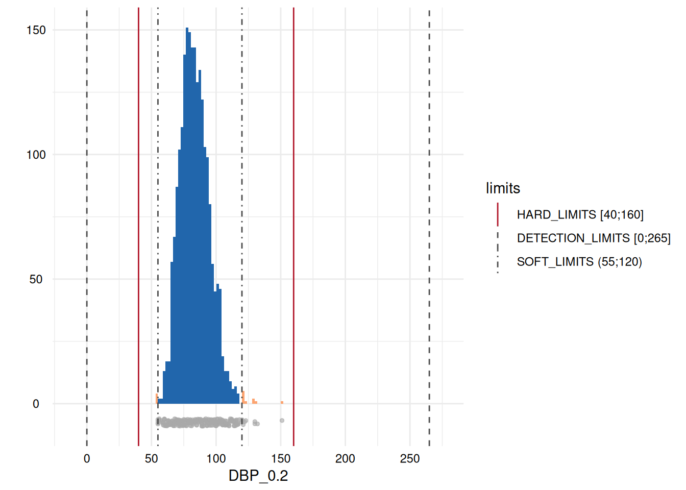
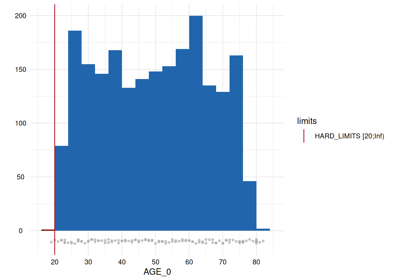
whichdeviate <- whichdeviate[!is.na(whichdeviate)]We can restrict the plots to those where variables have limit
deviations, i.e., those with a GRADING of 1 in the table above, using
MyValueLimits$SummaryPlotList[whichdeviate] (only the first
two are displayed below to reduce file size):