 Data Quality
Unexpected scale and shape
Assessing the shape of a distribution is, next to location
parameters, an important aspect of accuracy. Observed distributions can
be tested against expected distributions using the function acc_shape_or_scale.
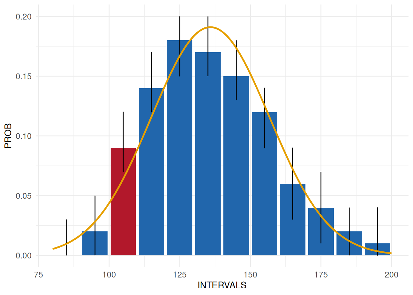
In this example the normal distribution of blood pressure is
examined:
# Load dataquieR
library(dataquieR)

# Load data
sd1 <- prep_get_data_frame("ship")

# Load metadata
prep_load_workbook_like_file("ship_meta_v2")
meta_data_item <- prep_get_data_frame("item_level") # item_level is a sheet in ship_meta_v2.xlsx

# Apply indicator function
MyUnexpDist2 <- acc_shape_or_scale(
  study_data = sd1,
  meta_data  = meta_data_item,
  resp_vars  = "SBP_0.2",
  guess      = TRUE,
  label_col  =  "LABEL",
  dist_col   = "DISTRIBUTION",
)

MyUnexpDist2$SummaryPlot
The result reveals a slight discrepancy from the normality assumption. It is up to the person responsible for the data quality assessments to decide whether such a discrepancy is relevant.
The analysis of end digit preferences is a specific implementation of
Unexpected shape. In this example,
the uniform distribution of the end digits of body height are examined
using acc_end_digits.
Body height in SHIP-START-0 was a measurement which required the manual
reading and transfer of data into an eCRF.
MyEndDigits <- acc_end_digits(
  study_data = sd1,
  meta_data  = meta_data_item,
  resp_vars  = "BODY_HEIGHT_0",
  label_col  = "LABEL"
)

MyEndDigits$SummaryPlot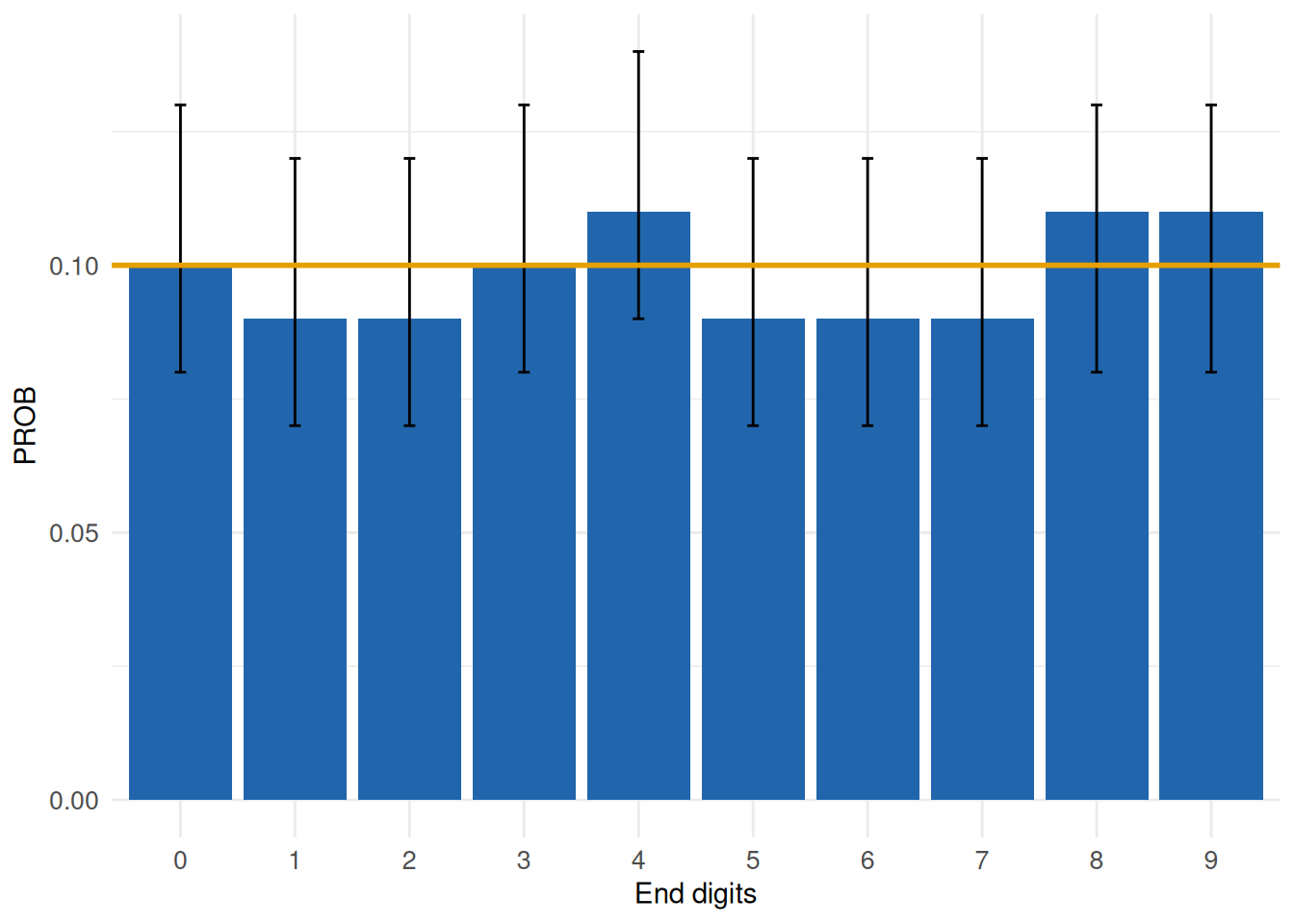
The graph highlights no relevant effects across the ten categories. Output within the accuracy dimension frequently combines descriptive and inferential content, which is necessary to facilitate valid conclusions on data quality issues. Further details on all functions can be obtained following the links and in the Software section.
