Data Quality
Univariate outliers
Univariate outliers are assessed
based on statistical criteria. The function acc_robust_univariate_outlier
identifies outliers according to the approaches of Tukey,
3SD,
Hubert,
and the heuristic approach of SigmaGap. It may be called as
follows:
# Load dataquieR
library(dataquieR)

# Load data
sd1 <- prep_get_data_frame("ship")

# Load metadata
prep_load_workbook_like_file("ship_meta_v2")
meta_data_item <- prep_get_data_frame("item_level") # item_level is a sheet in ship_meta_v2.xlsx

# Apply indicator function
UnivariateOutlier <- acc_robust_univariate_outlier(
  study_data = sd1,
  meta_data = meta_data_item,
  label_col = "LABEL"
)
The first output is a table that provides descriptive statistics and detected outliers according to the different criteria:
UnivariateOutlier$SummaryTable| Variables | Mean | No.records | SD | Median | Skewness | Tukey (N) | 3SD (N) | Hubert (N) | Sigma-gap (N) | NUM_acc_ud_outlu | Outliers, low (N) | Outliers, high (N) | GRADING | PCT_acc_ud_outlu |
|---|---|---|---|---|---|---|---|---|---|---|---|---|---|---|
| ID | 5431.06 | 2154 | 1236.17 | 5428.50 | 0.00 | 0 | 0 | 0 | 0 | 0 | 0 | 0 | 0 | 0.00 |
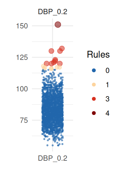
| DBP_0.2 | 83.52 | 2148 | 11.52 | 83.00 | 0.04 | 17 | 10 | 10 | 1 | 1 | 0 | 1 | 1 | 0.05 |
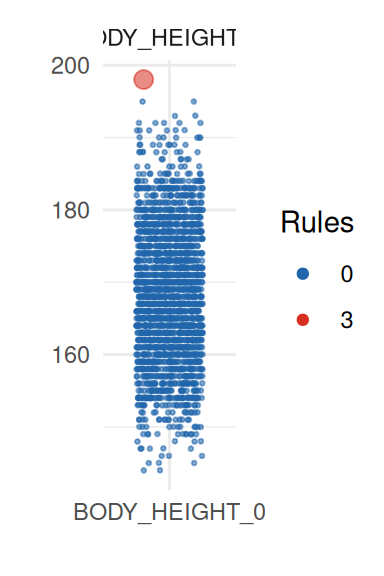
| BODY_HEIGHT_0 | 168.22 | 2151 | 9.25 | 168.00 | 0.00 | 1 | 1 | 1 | 0 | 0 | 0 | 0 | 0 | 0.00 |
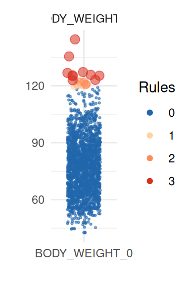
| BODY_WEIGHT_0 | 77.63 | 2150 | 15.08 | 77.04 | 0.01 | 17 | 10 | 15 | 0 | 0 | 0 | 0 | 0 | 0.00 |
| WAIST_CIRC_0 | 89.21 | 2148 | 13.82 | 89.52 | -0.05 | 6 | 6 | 15 | 0 | 0 | 0 | 0 | 0 | 0.00 |
| DIAB_AGE_ONSET_0 | 53.68 | 173 | 13.33 | 55.00 | 0.00 | 5 | 3 | 5 | 0 | 0 | 0 | 0 | 0 | 0.00 |
| CHOLES_HDL_0 | 1.45 | 2138 | 0.44 | 1.39 | 0.13 | 33 | 17 | 18 | 2 | 2 | 0 | 2 | 1 | 0.09 |
| CHOLES_LDL_0 | 3.58 | 2126 | 1.13 | 3.52 | 0.02 | 21 | 13 | 18 | 0 | 0 | 0 | 0 | 0 | 0.00 |
| CHOLES_ALL_0 | 5.76 | 2139 | 1.20 | 5.68 | 0.06 | 23 | 12 | 17 | 0 | 0 | 0 | 0 | 0 | 0.00 |
| AGE_0 | 49.87 | 2153 | 16.18 | 50.00 | -0.02 | 0 | 0 | 0 | 0 | 0 | 0 | 0 | 0 | 0.00 |
| SBP_0.1 | 138.25 | 2131 | 21.25 | 137.00 | 0.06 | 8 | 0 | 4 | 0 | 0 | 0 | 0 | 0 | 0.00 |
| SBP_0.2 | 135.87 | 2134 | 20.89 | 134.00 | 0.09 | 10 | 5 | 3 | 0 | 0 | 0 | 0 | 0 | 0.00 |
| DBP_0.1 | 84.43 | 2150 | 11.43 | 84.00 | 0.00 | 17 | 12 | 15 | 1 | 1 | 0 | 1 | 1 | 0.05 |
There are outliers according to at least two criteria in most variables, but only for the diastolic blood pressure variables (DBP_0.1 and DBP_0.2) two outliers have been detected using the Sigma-gap criterion.
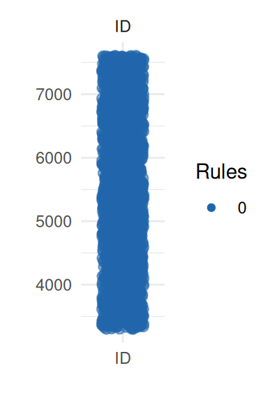
To obtain a better insight on univariate distributions, a plot is
provided (call it with UnivariateOutlier$SummaryPlotList).
It highlights observations for each variable according to the number of
violated rules (only the first four are shown here):
pl <- UnivariateOutlier$SummaryPlotList

invisible(lapply(head(pl, 4), print))