Data Quality
R implementation of distributional checks
Description
The function acc_distributions implements a range of
indicators and descriptors belonging to the Unexpected distributions domain in the
Accuracy dimension. It performs
location and proportion checks, as defined in the metadata, providing
data quality indicators for Unexpected
location and Unexpected
proportion.
Moreover, this implementation generates histograms (for float data
types) and bar plots (for integer data types), which are a frequent
approach to visualize the data distribution and possible data quality
issues. In this way, acc_distributions is also a descriptor
for Univariate outliers, Unexpected shape, and Unexpected scale. Note however, that for
outliers there exist dedicated functions to not only provide descriptors
but also outliers.
Usage and arguments
acc_distributions(
  resp_vars = NULL,
#  group_vars = NULL,
  label_col = "LABEL",
  study_data = sd1,
  meta_data = md1
)
The function has the following arguments:
- study_data: mandatory, the data frame containing the measurements.
- meta_data: mandatory, the data frame containing the item level metadata.
- resp_vars: optional, a character vector specifying the measurement variables of interest.
- group_vars: optional, the variable used for
grouping (e.g., observer or device). Defaults to
NULLfor output without grouping. deprecated, useacc_distributions_ecdf() - label_col: optional, the column in the metadata data frame containing the labels of all the variables in the study data.
acc_distributions_ecdf(
  resp_vars = NULL,
  group_vars = NULL,
  label_col = "LABEL",
  study_data = sd1,
  meta_data = md1
)
The function has the following arguments:
- study_data: mandatory, the data frame containing the measurements.
- meta_data: mandatory, the data frame containing the item level metadata.
- resp_vars: optional, a character vector specifying the measurement variables of interest.
- group_vars: optional, the variable used for
grouping (e.g., observer or device). Defaults to
NULLfor output without grouping. deprecated, useacc_distributions_ecdf() - label_col: optional, the column in the metadata data frame containing the labels of all the variables in the study data.
Example output
To illustrate the output, we use the example synthetic data and metadata that are bundled with the dataquieR package. See the introductory tutorial for instructions on importing these files into R, as well as details on their structure and contents.
To calculate the Unexpected
location and Unexpected
proportion indicators, the columns LOCATION_METRIC,
LOCATION_RANGE, and PROPORTION_RANGE, must be
specified in the metadata:
If the metadata does not contain these columns, the output will only provide distribution plots for the variables with float or integer data types.
Response variables without grouping variables
This is the simplest example, specifying only response variables
(SBP_0, for systolic blood pressure measurement,
SEX_0, and ITEM_4_0 of a questionnaire), the
study data, and the associated metadata:
dist_1 <- acc_distributions(
  resp_vars = c("SBP_0", "SEX_0", "ITEM_4_0"),
  label_col = "LABEL",
  study_data = sd1,
  meta_data = md1
)
Output 1: SummaryTable
acc_distributions returns three objects. The first two
data frames (SummaryTable and SummaryData)
contain the data quality checks for Unexpected location
(FLG_acc_ud_loc and VAL_acc_ud_loc) and Unexpected proportion for the response
variables. SummaryTable provides a concise summary of the
results, which is used by dq_report2 to populate the
accuracy section of the data quality report. Hence, the output is
minimal and the names of the columns are abbreviations. The
VAL columns give the calculated value(s) for unexpected
location or proportion, respectively. When an unexpected location or
proportion is found, the FLG columns provides a flag for
the corresponding variable. Call it with
dist_1$SummaryTable:
| Variables | values_from_data | GRADING | FLG_acc_ud_loc | loc_func | FLG_acc_ud_prop | prop_range |
|---|---|---|---|---|---|---|
| SBP_0 | 126.516204607575 | 0 | FALSE | mean | NA | NA |
| SEX_0 | females = 50.3 | males = 49.7 | 0 | NA | NA | FALSE | 0 in [48;52] |
| ITEM_4_0 | 0 = 4.9 | 1 = 14.2 | 2 = 22.9 | 3 = 23.3 | 4 = 16.6 | 5 = 10.3 | 6 = 4.2 | 7 = 2.1 | 8 = 1.1 | 9 = 0.3 | 10 = 0.1 | 1 | NA | NA | TRUE | 4 in (2;10] | 5 in (5;15] | 6 in (2;10] |
Output 2: SummaryData
The next output, SummaryData, presents the data quality
checks using explicit labels. It includes the response variable analysed
with its corresponding expected range and measure of location (specified
in the metadata), as reference. The columns Value and
Proportions show the calculated result, and according to
this, a binary flag is raised if values are outside the expectations.
Use dist_1$SummaryData to print the result:
| Variables | Range of expected values | Flag | Measure of location | Value | Proportions |
|---|---|---|---|---|---|
| SBP_0 | (100;140) | FALSE | mean | 126.5162 | NA |
| SEX_0 | 0 in [48;52] | FALSE | NA | NA | females = 50.3 | males = 49.7 |
| ITEM_4_0 | 4 in (2;10] | 5 in (5;15] | 6 in (2;10] | TRUE | NA | NA | 0 = 4.9 | 1 = 14.2 | 2 = 22.9 | 3 = 23.3 | 4 = 16.6 | 5 = 10.3 | 6 = 4.2 | 7 = 2.1 | 8 = 1.1 | 9 = 0.3 | 10 = 0.1 |
Output 3: SummaryPlotList
The last output contains a list of ggplots for each
variable in resp_vars. The plot shows the
LOCATION_RANGE or PROPORTION_RANGE as well as
the LOCATION_METRIC. Observations are highlighted if they
fall outside of the expected range.
dist_1$SummaryPlotList#[[1]]## $SBP_0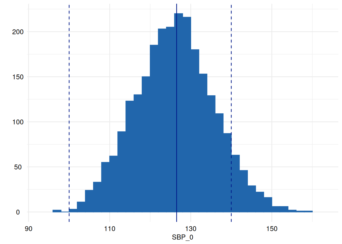
##
## $SEX_0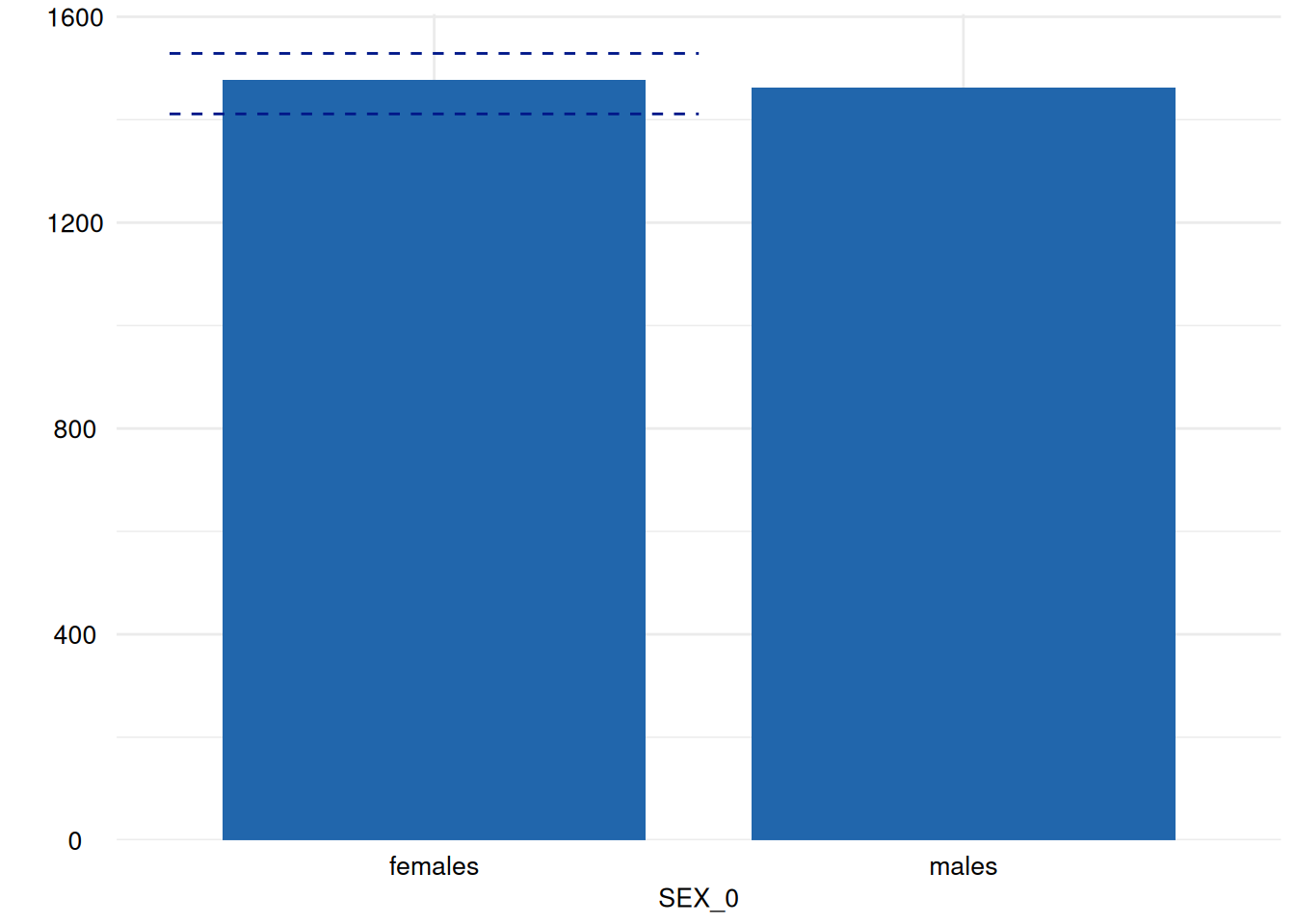
##
## $ITEM_4_0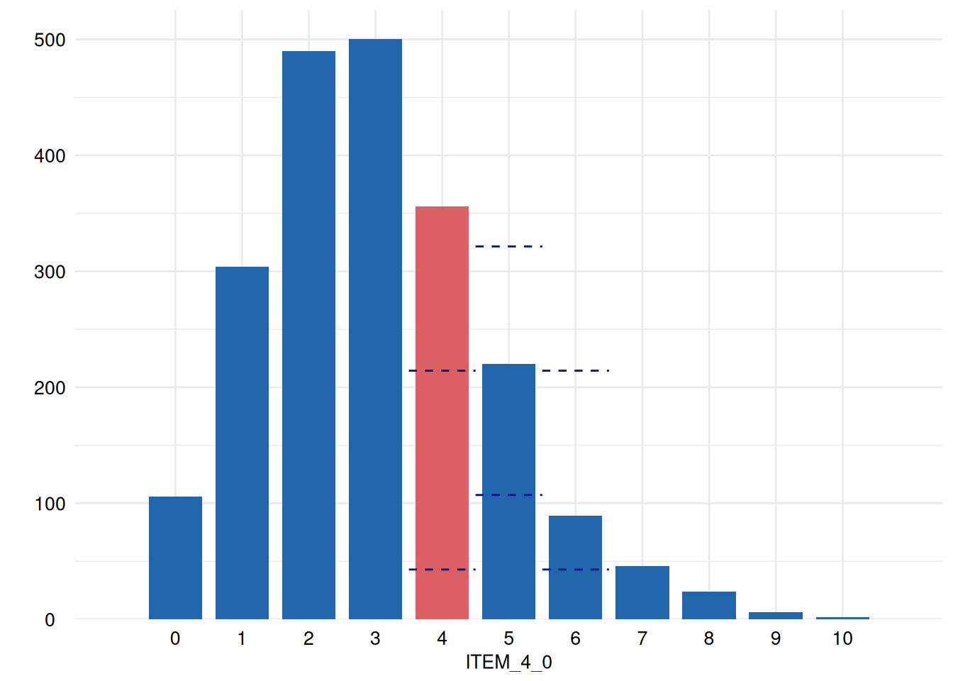
Response variables with a grouping variable
This example considers the SBP_0 (systolic blood
pressure measurement) with the grouping variable USR_BP_0
(examiner for the blood pressure measurement):
dist_2 <- acc_distributions_ecdf(
  resp_vars = "SBP_0",
  group_vars = "USR_BP_0",
  label_col = "LABEL",
  study_data = sd1,
  meta_data = md1
)
When the user specifies group_vars, the output
dist_2$SummaryPlotList includes a list of distribution
plots with their respective empirical Cumulative Distribution Function
(eCDF).
dist_2$SummaryPlotList#[[1]]## $SBP_0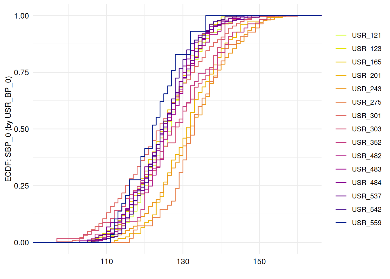
Interpretation
The higher the number of variables with unexpected location or proportions, the lower the data quality. Deviations from the expected central tendency or unexpected proportions might indicate data issues and should be further investigated.
Algorithm of the implementation
- If no response variable is defined, select all float or integer variables from the study data.
- Remove missing codes from the study data (if these are defined in the metadata).
- Remove measurements deviating from the (hard) limits (if these are defined in the metadata).
- Exclude variables containing only
NAor only one unique value (excludingNAs). - Perform check for Unexpected
location if defined in the metadata. This requires columns
LOCATION_METRIC(either mean or median) andLOCATION_RANGE(the range of expected values for the mean or median, respectively). - Perform check for Unexpected
proportion if defined in the metadata. This requires the column
PROPORTION_RANGE(the range of expected values for the proportions of the categories). (7)Plot histograms and bar charts. - If using
acc_distributions_ecdfandgroup_varsis specified by the user, output group-wise empirical cumulative distributions.
Because histogram classes are close to the density of the respective
distributions, instead of the default approach from
Sturges 1926,
acc_distributions uses the method of Freedman and Diaconis
(Freedman and Diaconis 1981) to define
the number of bins and breaks in histograms. The number of bins is
calculated as:
\[ No. \: of \: bins = 2* \frac{IQR(x)}{\sqrt[3] n} \]
If group_vars is given, the empirical Cumulative
Distribution Function (eCDF) is presented
(Drion et al.
1952).
For more details, see the user’s manual and source code.
Concept relations
- Data quality Indicator Unexpected location
- Data quality Indicator Unexpected proportion
- Data quality Indicator Unexpected scale
- Data quality Indicator Unexpected shape
- Data quality Indicator Univariate outliers