 Data Quality
R implementation of LOESS
Description
The acc_loess function conducts local regression (LOESS)
to examine the impact of so-called process variables on the
measurements over time
(Cleveland et al. 1988). In this way, the
acc_loess function is a descriptor for Unexpected location in the Unexpected distributions domain of the
Accuracy dimension. Moreover, it is
also a descriptor for Unexpected
association strength, Unexpected
association direction and Unexpected
association form, in the Unexpected
associations domain of the Accuracy dimension.
For more details, see the user’s manual and source code.
Usage and arguments
acc_loess(
  resp_vars = NULL,
  group_vars = NULL,
  time_vars = NULL,
  co_vars = NULL,
  min_obs_in_subgroup,
  label_col = NULL,
  study_data = sd1,
  meta_data = md1,
  resolution = 180,
  se_line = list(color = "red", linetype = 2),
  plot_data_time = NULL,
  plot_format = "AUTO"
)
The function has the following arguments:
- study_data: mandatory, the data frame containing the measurements.
- meta_data: mandatory, the data frame containing the item-level metadata.
- resp_vars: mandatory, a character specifying the continuous measurement variable of interest. The variable must be of float type.
- label_col: optional, the column in the metadata data frame containing the labels of all the variables in the study data.
- group_vars: optional, the variable used for
grouping (e.g., observer or device). Defaults to
NULLfor output without grouping. - time_variable: mandatory, a variable identifying the variable with the time of measurement.
- co_vars: optional, a vector of covariables, e.g. age and sex for adjustment.
- min_obs_level: optional, levels of the
group_varswith less measurements than defined inmin_obs_levelare excluded.
This implementation makes no use of a threshold. See Interpretation for guidance on the use of this function.
Example output
To illustrate the output, we use the example synthetic data and metadata that are bundled with the dataquieR package. See the introductory tutorial for instructions on importing these files into R, as well as details on their structure and contents.
Similar to the approach of the acc_margins function,
we assume that at least one examiner does not adhere to the SOP and may
influence the measurement process.
| v00000 | v00001 | v00002 | v00003 | v00004 | v00005 | v01003 | v01002 | v00103 | v00006 |
|---|---|---|---|---|---|---|---|---|---|
| 3 | LEIIX715 | 0 | 49 | 127 | 77 | 49 | 0 | 40-49 | 3.8 |
| 1 | QHNKM456 | 0 | 47 | 114 | 76 | 47 | 0 | 40-49 | 1.9 |
| 1 | HTAOB589 | 0 | 50 | 114 | 71 | 50 | 0 | 50-59 | 0.8 |
| 5 | HNHFV585 | 0 | 48 | 120 | 65 | 48 | 0 | 40-49 | 3.8 |
| 1 | UTDLS949 | 0 | 56 | 119 | 78 | 56 | 0 | 50-59 | 4.1 |
| 5 | YQFGE692 | 1 | 47 | 133 | 81 | 47 | 1 | 40-49 | 9.5 |
| 1 | AVAEH932 | 0 | 53 | 114 | 78 | 53 | 0 | 50-59 | 5.0 |
| 3 | QDOPT378 | 1 | 48 | 116 | 86 | 48 | 1 | 40-49 | 9.6 |
| 3 | BMOAK786 | 0 | 44 | 115 | 71 | 44 | 0 | 40-49 | 2.0 |
| 5 | ZDKNF462 | 0 | 50 | 116 | 74 | 50 | 0 | 50-59 | 2.4 |
For the acc_loess function, the columns
DATA_TYPE, MISSING_LIST and
HARD_LIMITS in the metadata are relevant.
| VAR_NAMES | LABEL | MISSING_LIST | DATA_TYPE | HARD_LIMITS | |
|---|---|---|---|---|---|
| 9 | v00004 | SBP_0 | 99980 | 99981 | 99982 | 99983 | 99984 | 99985 | 99986 | 99987 | 99988 | 99989 | 99990 | 99991 | 99992 | 99993 | 99994 | 99995 | float | [80;180] |
| 10 | v00005 | DBP_0 | 99980 | 99981 | 99982 | 99983 | 99984 | 99985 | 99986 | 99987 | 99988 | 99989 | 99990 | 99991 | 99992 | 99993 | 99994 | 99995 | float | [50;Inf) |
| 11 | v00006 | GLOBAL_HEALTH_VAS_0 | 99980 | 99983 | 99987 | 99988 | 99989 | 99990 | 99991 | 99992 | 99993 | 99994 | 99995 | float | [0;10] |
| 14 | v00009 | ARM_CIRC_0 | 99980 | 99981 | 99982 | 99983 | 99984 | 99985 | 99986 | 99987 | 99988 | 99989 | 99990 | 99991 | 99992 | 99993 | 99994 | 99995 | float | [0;Inf) |
| 21 | v00014 | CRP_0 | 99980 | 99981 | 99982 | 99983 | 99984 | 99985 | 99986 | 99988 | 99989 | 99990 | 99991 | 99992 | 99994 | 99995 | float | [0;Inf) |
| 22 | v00015 | BSG_0 | 99980 | 99981 | 99982 | 99983 | 99984 | 99985 | 99986 | 99988 | 99989 | 99990 | 99991 | 99992 | 99994 | 99995 | float | [0;100] |
The call of the function is illustrated here:
loess_1 <- acc_loess(
resp_vars = "SBP_0",
group_vars = "USR_BP_0",
time_vars = "EXAM_DT_0",
co_vars = c("AGE_0", "SEX_0"),
min_obs_in_subgroup = 30,
label_col = LABEL,
study_data = sd1,
meta_data = md1,
plot_format = "BOTH"
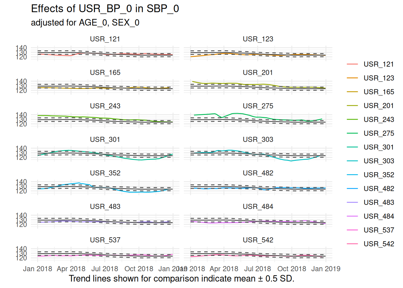
)The first plot is obtained by calling
loess_1$SummaryPlotList[[1]] and provides panels for each
subject/object. The plot contains LOESS-smoothed curves for each level
of the group_vars. The red dashed lines represent the
confidence interval of a LOESS curve for the whole data.
Output 1:
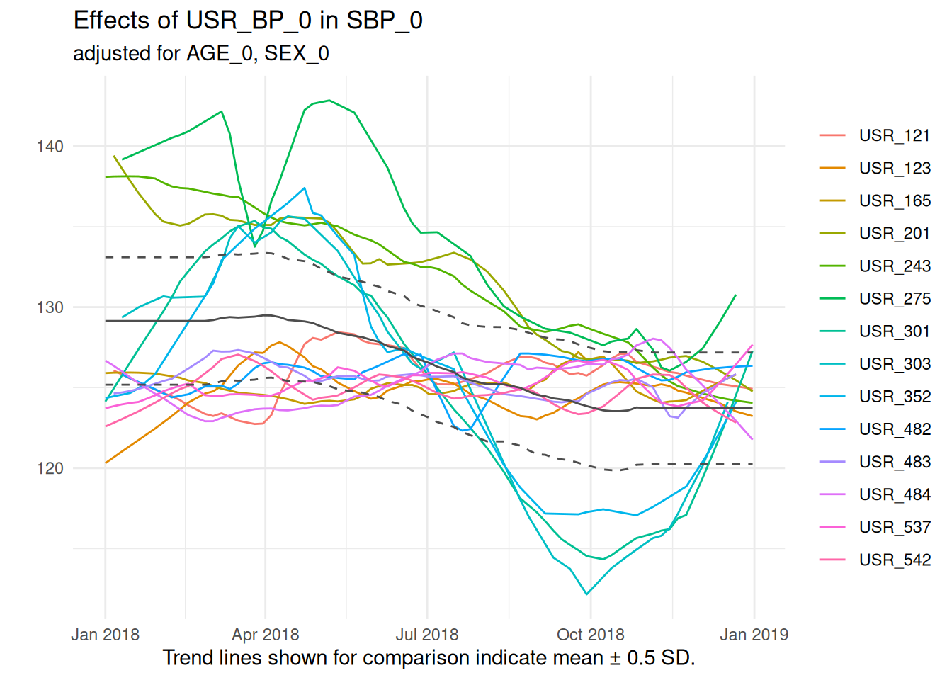
Output 2:
The second plot combines all levels of group_vars:
Interpretation
The following aspects should be considered when investigating the plots:
Random fluctuation
If changes in all levels of the group_vars appear at
random, no systematic trends over time are likely.
Seasonal trends
If seasonal trends such as sigmoidal curves are observed in one or
selected levels of the group_vars, intermittent location
shifts are observed.
Persistent trends
As shown in the example above for “USR_482”, persistent trends in one
or selected levels of the group_vars imply a systematic
change in measurements over time. If a fitted curve exceeds the
confidence band of dashed red lines of the overall distribution a severe
shift is observed.
Discrete processes
If for one level of the group_vars a complete separation
of the LOESS curve compared to all other levels is apparent, systematic
differences in measurements are likely which are independent of
time.
Algorithm of the implementation
- This implementation is yet restricted to data of type float.
- Missing codes are removed from
resp_vars(if defined in the metadata) - Deviations from limits, as defined in the metadata, are removed
- A linear model is estimated for
resp_varsusingco_varsfor adjustment. - The residuals of the model in (4) are used to fit LOESS for each
level of the
group_varsstatement along with date-values of atime_varsstatement. - A summary plot is generated for each level of
group_vars.
Limitations
The application of LOESS usually requires model fitting, i.e. the
smoothness of a model is subject to a smoothing parameter (span).
Particularly in the presence of interval-based missing data (USR_181),
high variability of measurements combined with a low number of
observations in one level of the group_vars the fit to the
data may be distorted. Since our approach handles data without knowledge
of such underlying characteristics, finding the best fit is complicated
if computational costs should be minimal. The default of LOESS in R uses
a span 0.75 which provides in most cases reasonable fits. The function
above increases the fit to the data automatically if the minimum of
observations in one level of the group_vars is higher than
30.
Concept relations
- Data quality Indicator Unexpected association direction
- Data quality Indicator Unexpected association form
- Data quality Indicator Unexpected association strength
- Data quality Indicator Unexpected location
