Unexpected location and proportion
Distributions
The function acc_distributions
examines Unexpected location and Unexpected proportion using histograms
and displays empirical cumulative distribution functions (ecdf) if a
grouping variable is provided.
The following example examines measurements in which a possible influence of the examiners is considered:
# Load dataquieR
library(dataquieR)

# Load data
sd1 <- prep_get_data_frame("ship")

# Load metadata
prep_load_workbook_like_file("ship_meta_v2")
meta_data_item <- prep_get_data_frame("item_level") # item_level is a sheet in ship_meta_v2.xlsx

# Apply indicator function
ECDFSoma1 <- acc_distributions(
  study_data = sd1,
  meta_data = meta_data_item,
  resp_vars = c("WAIST_CIRC_0", "BODY_HEIGHT_0", "BODY_WEIGHT_0"),
  label_col = "LABEL"
)
ECDFSoma2 <- acc_distributions_ecdf(
  study_data = sd1,
  meta_data = meta_data_item,
  resp_vars = c("WAIST_CIRC_0", "BODY_HEIGHT_0", "BODY_WEIGHT_0"),
  group_vars = "OBS_SOMA_0",
  label_col = "LABEL"
)
The respective list of plots may be displayed using
ECDFSoma1$SummaryPlotList /
ECDFSoma2$SummaryPlotList (only the first 2 plots are
displayed below):

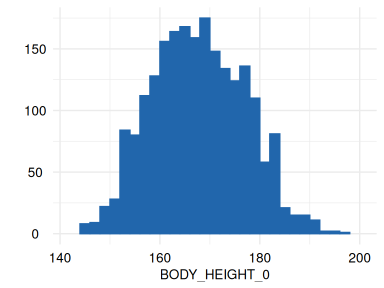
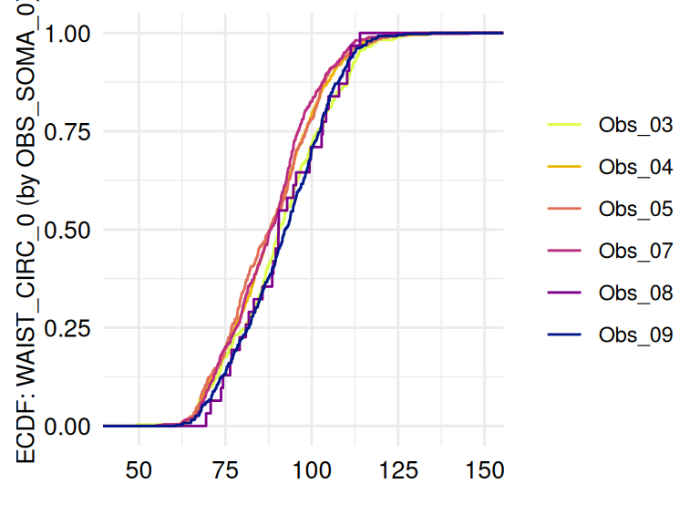
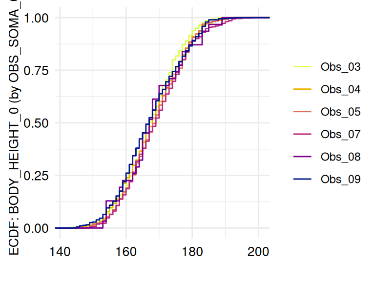
Marginal distributions
The function acc_margins is also
related to these indicators. However, it also provides descriptive
outputs, such as violin and box plots for continuous variables, count
plots for categorical data, and density plots for both. The main
application of acc_margins is to make
inference on effects related to process variables, such as examiners,
devices, or study centers. The function determines whether measurements
are continuous or discrete. Alternatively, this information may be
specified in the metadata.
In the example, acc_margins is applied
to the variable waist circumference (WAIST_CIRC_0). In this
case, dependencies related to the examiners (OBS_SOMA_0) are
assessed, while the raw measurements are controlled for variable age and
sex (AGE_0, SEX_0):
marginal_dists <- acc_margins(
  study_data      = sd1,
  meta_data       = meta_data_item,
  resp_vars  = "WAIST_CIRC_0",
  co_vars    = c("AGE_0", "SEX_0"),
  group_vars = "OBS_SOMA_0",
  label_col  = "LABEL"
)
A plot is provided to view the results:
marginal_dists$SummaryPlot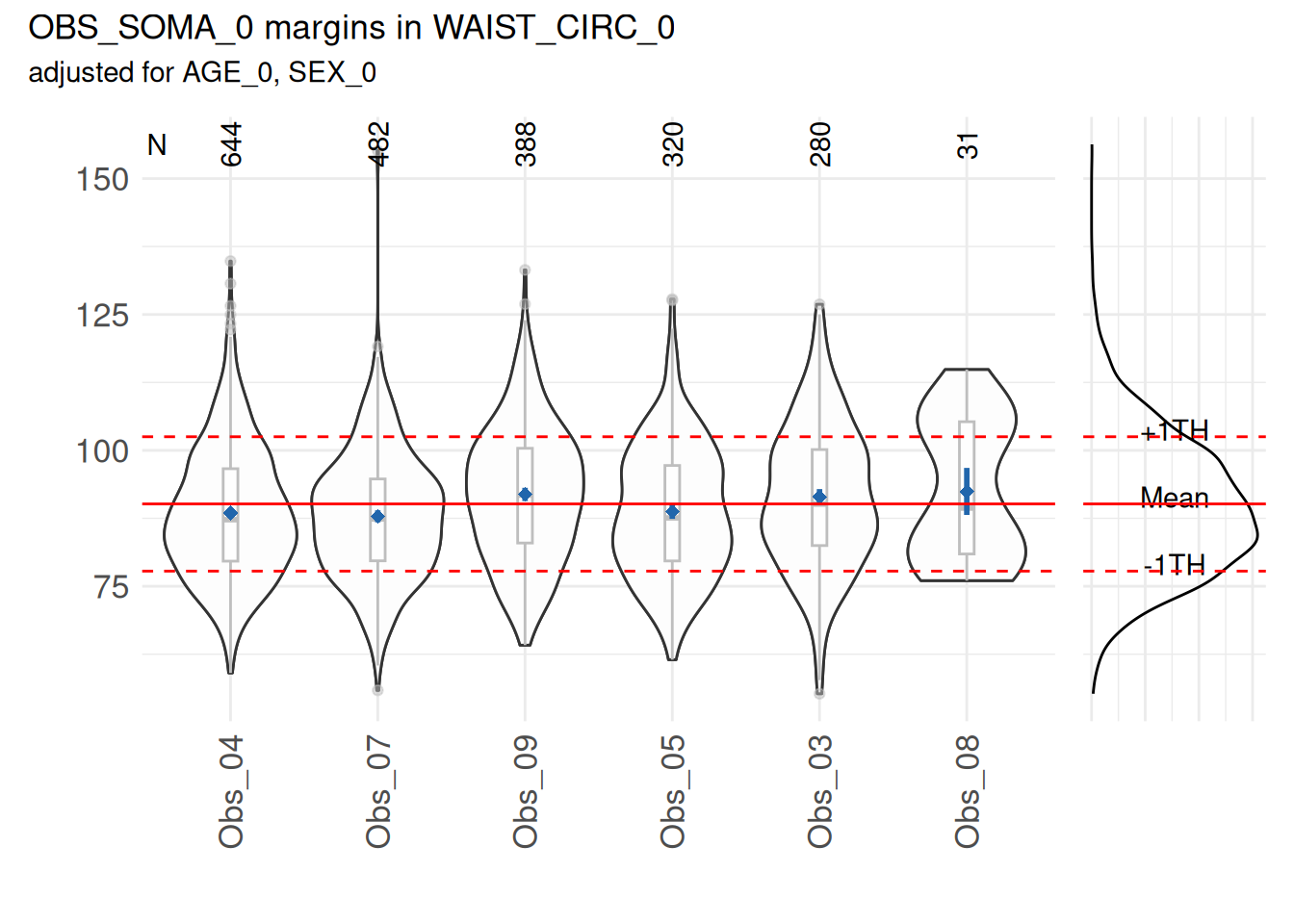
Based on a statistical test, no mean waist circumference of any examiner differed substantially (p<0.05) from the overall mean.
However, some examiners can have a mean that differ from the overall mean. This can be observed in the following example, where the measurements of waist circumference of the examiner “3” have been increased by 20.
#increase by 20 the measurements of observer 3
sd1_example <- dplyr::mutate(sd1, waist= ifelse(obs_soma == "3", as.numeric(waist)+20, waist))

marginal_dists <- acc_margins(
    study_data      = sd1_example ,
    meta_data       = meta_data_item,
    resp_vars  = "WAIST_CIRC_0",
    co_vars    = c("AGE_0", "SEX_0"),
    group_vars = "OBS_SOMA_0",
    label_col  = "LABEL"
)

marginal_dists$SummaryPlot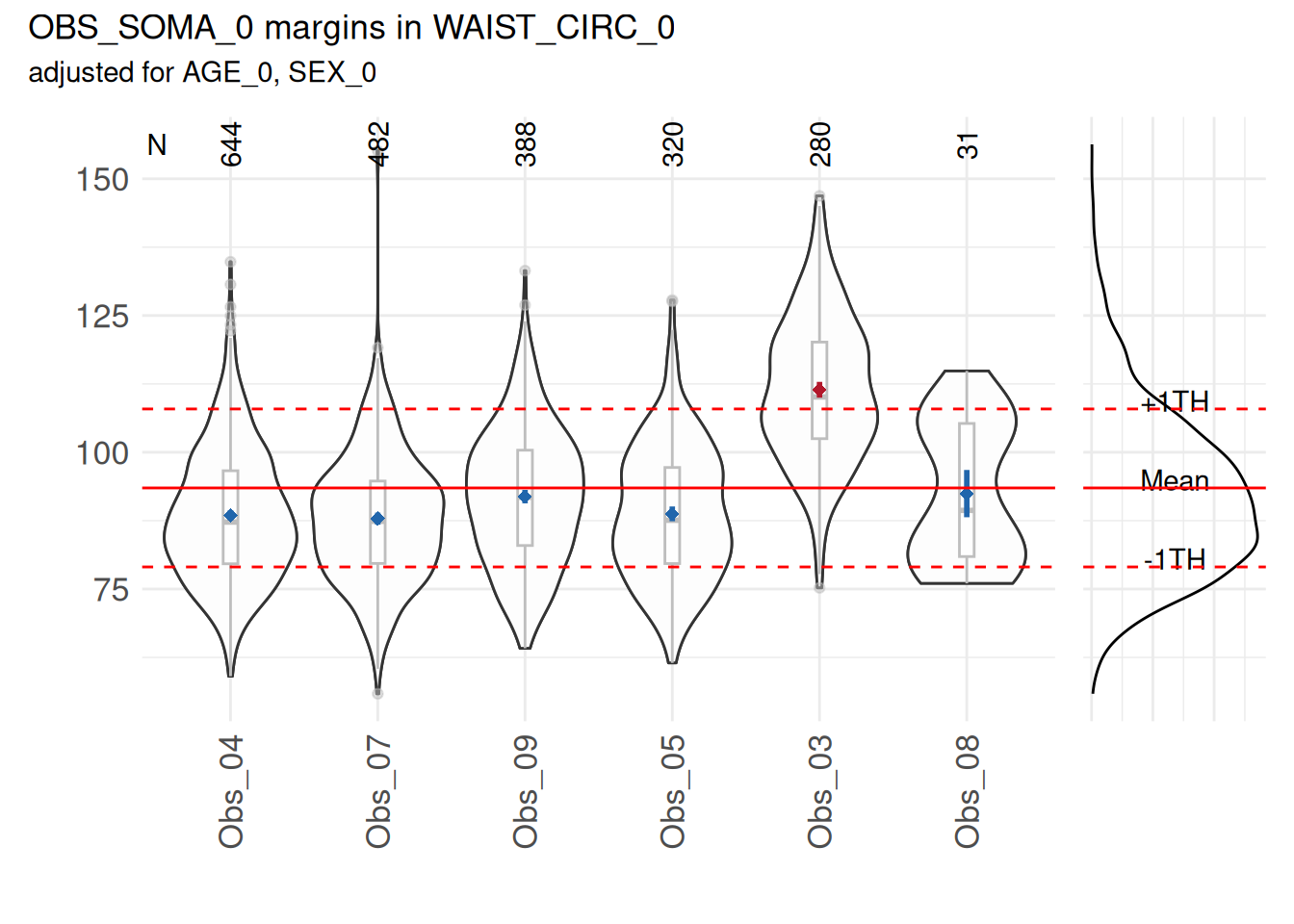
The result shows elevated proportions for the examiner 03.
LOESS
The study of effects across groups and times is particularly complex.
The function acc_loess provides a
descriptor related to the indicator Unexpected location. acc_loess may also be
used to obtain information related to other indicators in the domain of
unexpected distributions.
An example call using waist circumference as the target variable is:
timetrends <- acc_loess(
  study_data = sd1,
  meta_data  = meta_data_item,
  resp_vars  = "WAIST_CIRC_0",
  co_vars    = c("AGE_0", "SEX_0"),
  group_vars = "OBS_SOMA_0",
  time_vars  = "EXAM_DT_0",
  label_col  = "LABEL"
)

invisible(lapply(timetrends$SummaryPlotList, print))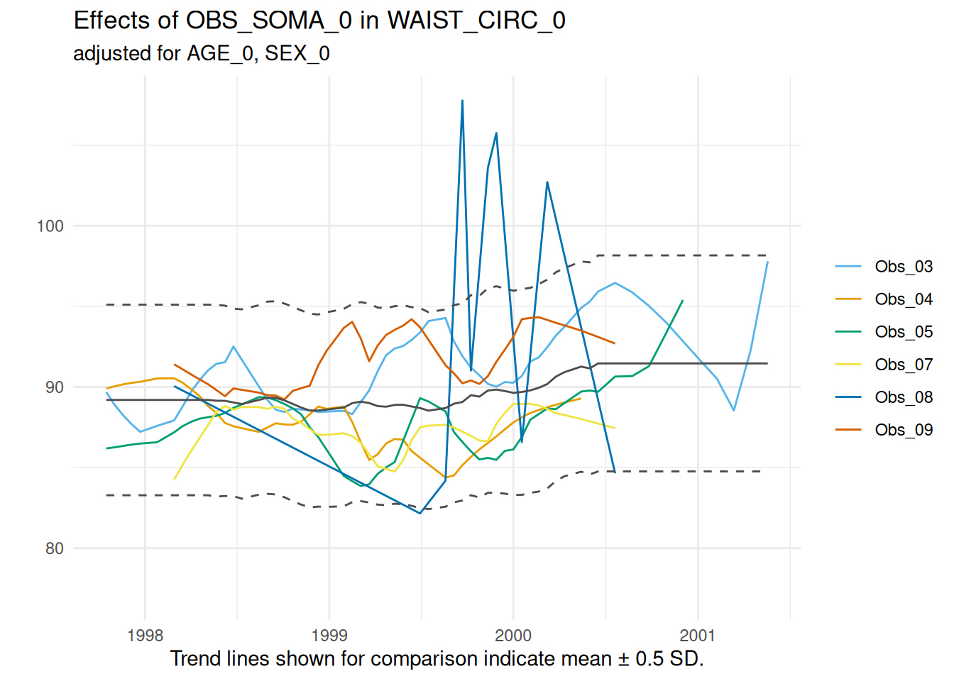
The graph for this variable indicates no major discrepancies between the examiners over the examination period.
 Data Quality


