 Data Quality
Item level data quality assessment example
Introduction
Data quality assessments at the level of single data elements
(variables/items) require item
level metadata.
These metadata are needed to address the compliance of study data with
expectations, the occurrence and patterns of missing data, the presence
of inadmissible or uncertain numerical or categorical values, the
presence of univariate or multivariate outliers, and the variance
proportion explained by different groups (e.g. devices). Item level
metadata are also needed to describe the agreement between observed and
expected distributions. This tutorial shows how to compute data quality
indicators at the item level using dataquieR.
Example data
To illustrate the functionalities, we use a subset of the example SHIP data and metadata that are bundled with the dataquieR package. See the introductory tutorial for instructions on importing these files into R, as well as details on their structure and contents.
The basic workflow is:
library(dataquieR)
sd1 <- prep_get_data_frame("ship")
sd1 <- as.data.frame(sd1) # "untibble" it
The study data consists of:
- N = 2154 observations, and
- P = 33 study variables.
Required metadata
To evaluate data quality at the item level, we must provide descriptions and expectations about the variables in dataquieR’s metadata format. For instance, for the SHIP example data, the metadata may be imported as follows:
prep_load_workbook_like_file("ship_meta_v2")
meta_data_item <- prep_get_data_frame("item_level") # item_level is a sheet in ship_meta_v2.xlsx
The imported metadata provides information for:
- P = 33 study variables, and
- Q = 27 variable level attributes.
An identical number of variables in the study data and metadata is desirable but not necessary. Columns in the metadata include information on each variable of the study data file, such as labels or admissibility limits:
| VAR_NAMES | LABEL | DATA_TYPE | SCALE_LEVEL | VALUE_LABELS | STANDARDIZED_VOCABULARY_TABLE | MISSING_LIST_TABLE | HARD_LIMITS | DETECTION_LIMITS | SOFT_LIMITS | DISTRIBUTION | DECIMALS | END_DIGIT_CHECK | GROUP_VAR_OBSERVER | GROUP_VAR_DEVICE | TIME_VAR | STUDY_SEGMENT | DATAFRAMES | VARIABLE_ROLE | VARIABLE_ORDER | LONG_LABEL | UNIVARIATE_OUTLIER_CHECKTYPE | N_RULES | LOCATION_METRIC | LOCATION_RANGE | PROPORTION_RANGE | CO_VARS |
|---|---|---|---|---|---|---|---|---|---|---|---|---|---|---|---|---|---|---|---|---|---|---|---|---|---|---|
| id | ID | integer | na | NA | NA | NA | NA | NA | NA | NA | NA | NA | NA | NA | NA | INTRO | SHIP | intro | 1 | Participant ID | NA | 4 | NA | NA | NA | NA |
| exdate | EXAM_DT_0 | datetime | interval | NA | NA | NA | [1995-01-01;) | NA | NA | NA | NA | NA | NA | NA | NA | INTRO | SHIP | process | 2 | Examination date and time | NA | 4 | NA | NA | NA | NA |
| sex | SEX_0 | integer | nominal | 1 = males | 2 = females | NA | NA | NA | NA | NA | NA | NA | NA | NA | NA | NA | INTRO | SHIP | intro | 3 | Sex | NA | 4 | NA | NA | (48;52) | NA |
| age | AGE_0 | integer | ratio | NA | NA | NA | [20;Inf) | NA | NA | NA | NA | NA | NA | NA | NA | INTRO | SHIP | intro | 4 | Age | NA | 4 | NA | NA | NA | NA |
| obs_bp | OBS_BP_0 | integer | nominal | 1 = Obs_01 | 2 = Obs_02 | 3 = Obs_03 | 4 = Obs_04 | 5 = Obs_05 | 6 = Obs_06 | 7 = Obs_07 | 8 = Obs_08 | 9 = Obs_09 | 10 = Obs_10 | 11 = Obs_11 | 12 = Obs_12 | 13 = Obs_13 | 14 = Obs_14 | 15 = Obs_15 | 16 = Obs_16 | 17 = Obs_17 | 18 = Obs_18 | 19 = Obs_19 | 20 = Obs_20 | NA | missing_table | NA | NA | NA | NA | NA | NA | NA | NA | NA | SOMATOMETRY | SHIP | process | 5 | Blood pressure examiner | NA | 4 | NA | NA | NA | NA |
| dev_bp | DEV_BP_0 | integer | nominal | 1 = Dev_01 | 2 = Dev_02 | 3 = Dev_03 | 4 = Dev_04 | 5 = Dev_05 | 6 = Dev_06 | 7 = Dev_07 | 8 = Dev_08 | 9 = Dev_09 | 10 = Dev_10 | 11 = Dev_11 | 12 = Dev_12 | 13 = Dev_13 | 14 = Dev_14 | 15 = Dev_15 | 16 = Dev_16 | 17 = Dev_17 | 18 = Dev_18 | 19 = Dev_19 | 20 = Dev_20 | 21 = Dev_21 | 22 = Dev_22 | 23 = Dev_23 | 24 = Dev_24 | 25 = Dev_25 | NA | missing_table | NA | NA | NA | uniform | NA | NA | NA | NA | NA | SOMATOMETRY | SHIP | process | 6 | Blood pressure device ID | NA | 4 | NA | NA | NA | NA |
| sbp1 | SBP_0.1 | integer | ratio | NA | NA | NA | [80;200] | [0;265] | (90;180) | normal | NA | NA | obs_bp | dev_bp | exdate | SOMATOMETRY | SHIP | primary | 7 | Systolic blood pressure 1 | NA | 4 | Mean | (100;140) | NA | sex | age |
| sbp2 | SBP_0.2 | integer | ratio | NA | NA | NA | [80;200] | [0;265] | (90;180) | normal | NA | NA | obs_bp | dev_bp | exdate | SOMATOMETRY | SHIP | primary | 8 | Systolic blood pressure 2 | NA | 4 | Mean | (100;140) | NA | sex | age |
| dbp1 | DBP_0.1 | integer | ratio | NA | NA | NA | [40;160] | [0;265] | (55;120) | normal | NA | NA | obs_bp | dev_bp | exdate | SOMATOMETRY | SHIP | primary | 9 | Diastolic blood pressure 1 | NA | 4 | Mean | (60;100) | NA | sex | age |
| dbp2 | DBP_0.2 | integer | ratio | NA | NA | NA | [40;160] | [0;265] | (55;120) | normal | NA | NA | obs_bp | dev_bp | exdate | SOMATOMETRY | SHIP | primary | 10 | Diastolic blood pressure 2 | NA | 4 | Mean | (60;100) | NA | sex | age |
| obs_soma | OBS_SOMA_0 | integer | nominal | 1 = Obs_01 | 2 = Obs_02 | 3 = Obs_03 | 4 = Obs_04 | 5 = Obs_05 | 6 = Obs_06 | 7 = Obs_07 | 8 = Obs_08 | 9 = Obs_09 | 10 = Obs_10 | NA | missing_table | NA | NA | NA | NA | NA | NA | NA | NA | NA | SOMATOMETRY | SHIP | process | 11 | Somatometry examiner | NA | 4 | NA | NA | 1 = [0;5) | 2 = [0;5) | 3 = [15;30] | 4 = [15;30] | 5 = [15;30] | 6 = [0;5) | 7 = [15;30] | 8 = [0;5) | 9 = [15;30] | 10 = [0;5) | NA |
| height | BODY_HEIGHT_0 | integer | ratio | NA | NA | missing_table | [80;230] | NA | NA | NA | 1 | 1 | obs_soma | dev_length | exdate | SOMATOMETRY | SHIP | primary | 12 | Body height | NA | 4 | NA | NA | NA | NA |
| dev_length | DEV_HEIGHT_0 | integer | nominal | 1 = Dev_01 | 2 = Dev_02 | 3 = Dev_03 | 4 = Dev_04 | 5 = Dev_05 | 6 = Dev_06 | 7 = Dev_07 | 8 = Dev_08 | 9 = Dev_09 | 10 = Dev_10 | 11 = Dev_11 | 12 = Dev_12 | 13 = Dev_13 | 14 = Dev_14 | 15 = Dev_15 | 16 = Dev_16 | 17 = Dev_17 | 18 = Dev_18 | 19 = Dev_19 | 20 = Dev_20 | 21 = Dev_21 | 22 = Dev_22 | 23 = Dev_23 | 24 = Dev_24 | 25 = Dev_25 | NA | missing_table | NA | NA | NA | NA | NA | NA | NA | NA | NA | SOMATOMETRY | SHIP | process | 13 | Body height scale ID | NA | 4 | NA | NA | NA | NA |
| weight | BODY_WEIGHT_0 | float | ratio | NA | NA | missing_table | [30;250] | NA | NA | NA | 2 | 1 | obs_soma | dev_weight | exdate | SOMATOMETRY | SHIP | primary | 14 | Body weight | NA | 4 | NA | NA | NA | NA |
| dev_weight | DEV_WEIGHT_0 | integer | nominal | 1 = Dev_01 | 2 = Dev_02 | 3 = Dev_03 | 4 = Dev_04 | 5 = Dev_05 | 6 = Dev_06 | 7 = Dev_07 | 8 = Dev_08 | 9 = Dev_09 | 10 = Dev_10 | 11 = Dev_11 | 12 = Dev_12 | 13 = Dev_13 | 14 = Dev_14 | 15 = Dev_15 | 16 = Dev_16 | 17 = Dev_17 | 18 = Dev_18 | 19 = Dev_19 | 20 = Dev_20 | 21 = Dev_21 | 22 = Dev_22 | 23 = Dev_23 | 24 = Dev_24 | 25 = Dev_25 | NA | missing_table | NA | NA | NA | NA | NA | NA | NA | NA | NA | SOMATOMETRY | SHIP | process | 15 | Body weight scale ID | NA | 4 | NA | NA | NA | NA |
| waist | WAIST_CIRC_0 | float | ratio | NA | NA | missing_table | [30;Inf) | NA | NA | NA | NA | NA | obs_soma | NA | exdate | SOMATOMETRY | SHIP | primary | 16 | Waist circumference | NA | 4 | NA | NA | NA | NA |
| obs_int | OBS_INT_0 | integer | nominal | 1 = Obs_01 | 2 = Obs_02 | 3 = Obs_03 | 4 = Obs_04 | 5 = Obs_05 | 6 = Obs_06 | 7 = Obs_07 | 8 = Obs_08 | 9 = Obs_09 | 10 = Obs_10 | 11 = Obs_11 | 12 = Obs_12 | 13 = Obs_13 | 14 = Obs_14 | 15 = Obs_15 | 16 = Obs_16 | 17 = Obs_17 | 18 = Obs_18 | 19 = Obs_19 | 20 = Obs_20 | 21 = Obs_21 | 22 = Obs_22 | 23 = Obs_23 | 24 = Obs_24 | 25 = Obs_25 | NA | missing_table | NA | NA | NA | NA | NA | NA | obs_int | NA | NA | INTERVIEW | SHIP | process | 17 | Interview examiner | NA | 4 | NA | NA | NA | NA |
| school | SCHOOL_GRAD_0 | integer | ordinal | 0 = none | 1 = lower secondary | 2 = secondary | 3 = upper secondary | NA | missing_table | NA | NA | NA | NA | NA | NA | obs_int | NA | exdate | INTERVIEW | SHIP | primary | 18 | Highest educational level | NA | 4 | NA | NA | NA | NA |
| family | RELATION_STATUS_0 | integer | nominal | 1 = married | 2 = married (living apart) | 3 = single (never married) | 4 = divorced | 5 = widowed | NA | missing_table | NA | NA | NA | NA | NA | NA | obs_int | NA | exdate | INTERVIEW | SHIP | primary | 19 | Marital status | NA | 4 | NA | NA | NA | NA |
| smoking | SMOKING_STATUS_0 | integer | nominal | 0 = nonsmoker | 1 = former smoker | 2 = smoker | NA | missing_table | NA | NA | NA | NA | NA | NA | obs_int | NA | exdate | INTERVIEW | SHIP | primary | 20 | Smoking status | NA | 4 | NA | NA | NA | NA |
| stroke | STROKE_YN_0 | integer | nominal | 1 = yes | 2 = no | NA | missing_table | NA | NA | NA | NA | NA | NA | obs_int | NA | exdate | INTERVIEW | SHIP | primary | 21 | Ever had stroke | NA | 4 | NA | NA | NA | NA |
| myocard | MYOCARD_YN_0 | integer | nominal | 1 = yes | 2 = no | NA | missing_table | NA | NA | NA | NA | NA | NA | obs_int | NA | exdate | INTERVIEW | SHIP | primary | 22 | Ever had myocardial infarction | NA | 4 | NA | NA | NA | NA |
| diab_known | DIABETES_KNOWN_0 | integer | nominal | 0 = no | 1 = yes | NA | missing_table | NA | NA | NA | NA | NA | NA | obs_int | NA | exdate | INTERVIEW | SHIP | primary | 23 | Known diabetes | NA | 4 | NA | NA | NA | NA |
| diab_age | DIAB_AGE_ONSET_0 | integer | ratio | NA | NA | missing_table | NA | NA | NA | NA | NA | NA | obs_int | NA | exdate | INTERVIEW | SHIP | primary | 24 | Age of diabetes onset | NA | 4 | NA | NA | NA | NA |
| contraception | CONTRACEPTIVA_EVER_0 | integer | nominal | 1 = yes | 2 = no | NA | missing_table | NA | NA | NA | NA | NA | NA | obs_int | NA | exdate | INTERVIEW | SHIP | primary | 25 | Ever taken birth control pills | NA | 4 | NA | NA | NA | NA |
| income | HOUSE_INCOME_MONTH_0 | integer | ordinal | 1 = below 2000 | 2 = 2000 - 4000 | 3 = above 4000 | NA | missing_table | NA | NA | NA | NA | NA | NA | obs_int | NA | exdate | INTERVIEW | SHIP | primary | 26 | Monthly household income | NA | 4 | NA | NA | NA | NA |
| hdl | CHOLES_HDL_0 | float | ratio | NA | NA | missing_table | [0;Inf) | NA | NA | gamma | 3 | NA | NA | NA | exdate | LABORATORY | SHIP | primary | 27 | HDL-cholesterol | NA | 4 | NA | NA | NA | NA |
| ldl | CHOLES_LDL_0 | float | ratio | NA | NA | missing_table | [0;Inf) | NA | NA | gamma | 3 | NA | NA | NA | exdate | LABORATORY | SHIP | primary | 28 | LDL-cholesterol | NA | 4 | NA | NA | NA | NA |
| cholesterol | CHOLES_ALL_0 | float | ratio | NA | NA | missing_table | [0;Inf) | NA | NA | gamma | 3 | NA | NA | NA | exdate | LABORATORY | SHIP | primary | 29 | Total cholesterol | NA | 4 | NA | NA | NA | NA |
| seg_part_intro | SEG_PART_INTRO | integer | na | NA | NA | segment_missing_table | NA | NA | NA | NA | NA | NA | NA | NA | NA | INTRO | SHIP | intro | 30 | Intro segment consent | NA | 4 | NA | NA | NA | NA |
| seg_part_somatometry | SEG_PART_SOMATOMETRY | integer | na | NA | NA | segment_missing_table | NA | NA | NA | NA | NA | NA | NA | NA | NA | INTRO | SHIP | intro | 31 | Somatometry segment consent | NA | 4 | NA | NA | NA | NA |
| seg_part_interview | SEG_PART_INTERVIEW | integer | na | NA | NA | segment_missing_table | NA | NA | NA | NA | NA | NA | NA | NA | NA | INTRO | SHIP | intro | 32 | Interview segment consent | NA | 4 | NA | NA | NA | NA |
| seg_part_laboratory | SEG_PART_LABORATORY | integer | na | NA | NA | segment_missing_table | NA | NA | NA | NA | NA | NA | NA | NA | NA | INTRO | SHIP | intro | 33 | Laboratory segment consent | NA | 4 | NA | NA | NA | NA |
Note: The item level metadata file is the primary point of reference for generating data quality reports:
- It defines the number of variables for which to generate reports.
- It is the expected truth against which the study data are compared to.
A detailed description of how to set up this metadata file is available here. See here for an overview of dataquieR’s metadata usage.
Data quality indicators at the item level
The indicators at the item level are related to all data quality dimensions. These are described in detail in this tutorial. See the documentation of each function for an in-depth explanation of its usage.
Example usage and output
Integrity
The first step in the data quality assessment workflow evaluates the compliance of the study data to the respective metadata regarding formal and structural requirements.
Data type mismatch
The Data
type mismatch indicator be calculated using int_datatype_matrix
in the following way:
datatype_res <- int_datatype_matrix(
  study_data = sd1,
  meta_data = meta_data_item,
  label_col = "LONG_LABEL"
)
A plot and a table are provided to view the results:
datatype_res$SummaryPlot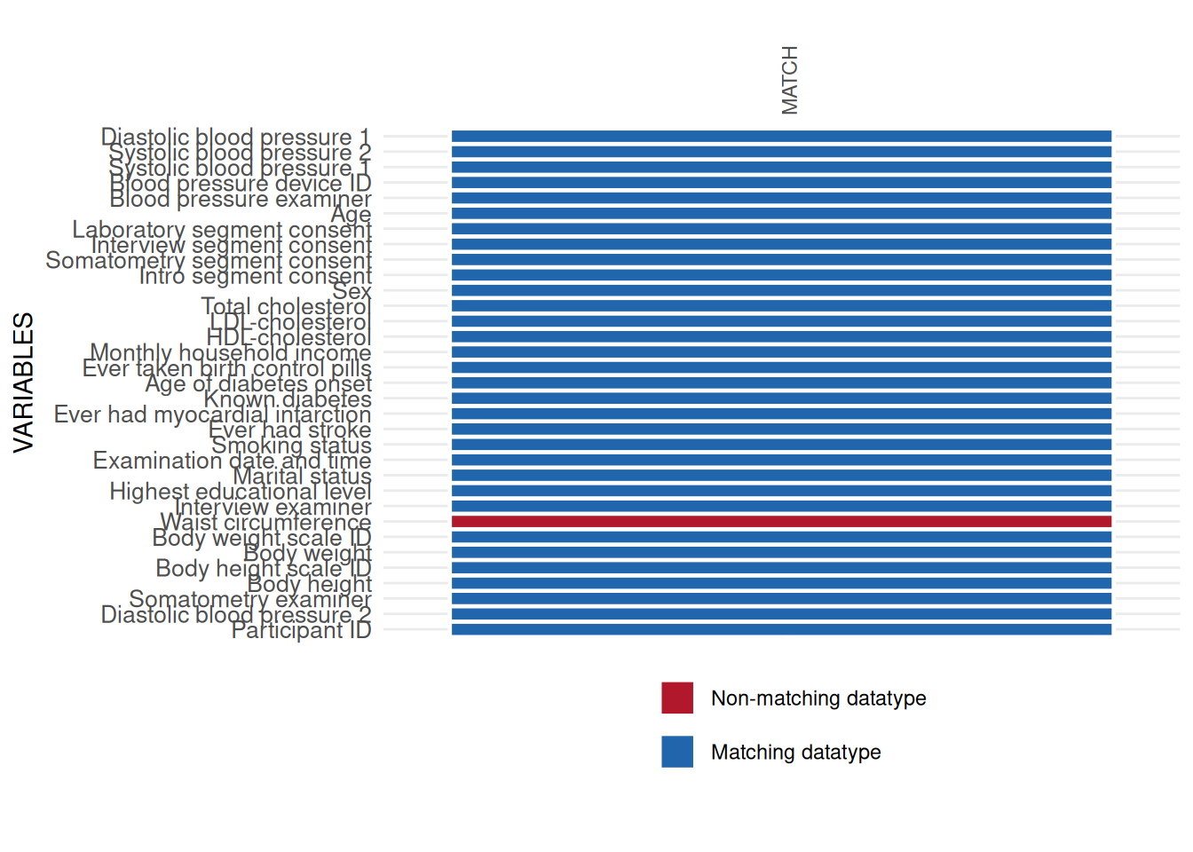
datatype_res$SummaryData| Variables | Data type mismatch N (%) | Convertible mismatch, stable N (%) | Convertible mismatch, unstable N (%) | Data type match N (%) | Expected DATA_TYPE | Observed DATA_TYPE | State, given threshold | STUDY_SEGMENT | |
|---|---|---|---|---|---|---|---|---|---|
| 25 | Participant ID | 0 (0.00%) | 0 ( 0.00%) | 0 (0.00%) | 2154 (100.00%) | integer | integer | Matching datatype | INTRO |
| 10 | Diastolic blood pressure 2 | 0 (0.00%) | 0 ( 0.00%) | 0 (0.00%) | 2154 (100.00%) | integer | integer | Matching datatype | SOMATOMETRY |
| 28 | Somatometry examiner | 0 (0.00%) | 0 ( 0.00%) | 0 (0.00%) | 2154 (100.00%) | integer | integer | Matching datatype | SOMATOMETRY |
| 5 | Body height | 0 (0.00%) | 0 ( 0.00%) | 0 (0.00%) | 2154 (100.00%) | integer | integer | Matching datatype | SOMATOMETRY |
| 6 | Body height scale ID | 0 (0.00%) | 0 ( 0.00%) | 0 (0.00%) | 2154 (100.00%) | integer | integer | Matching datatype | SOMATOMETRY |
| 7 | Body weight | 0 (0.00%) | 0 ( 0.00%) | 0 (0.00%) | 2154 (100.00%) | float | float | Matching datatype | SOMATOMETRY |
| 8 | Body weight scale ID | 0 (0.00%) | 0 ( 0.00%) | 0 (0.00%) | 2154 (100.00%) | integer | integer | Matching datatype | SOMATOMETRY |
| 33 | Waist circumference | 3 (0.14%) | 2148 ( 99.72%) | 0 (0.00%) | 3 ( 0.14%) | float | string | Non-matching datatype | SOMATOMETRY |
| 17 | Interview examiner | 0 (0.00%) | 0 ( 0.00%) | 0 (0.00%) | 2154 (100.00%) | integer | integer | Matching datatype | INTERVIEW |
| 16 | Highest educational level | 0 (0.00%) | 0 ( 0.00%) | 0 (0.00%) | 2154 (100.00%) | integer | integer | Matching datatype | INTERVIEW |
| 23 | Marital status | 0 (0.00%) | 0 ( 0.00%) | 0 (0.00%) | 2154 (100.00%) | integer | integer | Matching datatype | INTERVIEW |
| 14 | Examination date and time | 0 (0.00%) | 0 ( 0.00%) | 0 (0.00%) | 2154 (100.00%) | datetime | datetime | Matching datatype | INTRO |
| 27 | Smoking status | 0 (0.00%) | 0 ( 0.00%) | 0 (0.00%) | 2154 (100.00%) | integer | integer | Matching datatype | INTERVIEW |
| 12 | Ever had stroke | 0 (0.00%) | 0 ( 0.00%) | 0 (0.00%) | 2154 (100.00%) | integer | integer | Matching datatype | INTERVIEW |
| 11 | Ever had myocardial infarction | 0 (0.00%) | 0 ( 0.00%) | 0 (0.00%) | 2154 (100.00%) | integer | integer | Matching datatype | INTERVIEW |
| 20 | Known diabetes | 0 (0.00%) | 0 ( 0.00%) | 0 (0.00%) | 2154 (100.00%) | integer | integer | Matching datatype | INTERVIEW |
| 2 | Age of diabetes onset | 0 (0.00%) | 0 ( 0.00%) | 0 (0.00%) | 2154 (100.00%) | integer | integer | Matching datatype | INTERVIEW |
| 13 | Ever taken birth control pills | 0 (0.00%) | 0 ( 0.00%) | 0 (0.00%) | 2154 (100.00%) | integer | integer | Matching datatype | INTERVIEW |
| 24 | Monthly household income | 0 (0.00%) | 0 ( 0.00%) | 0 (0.00%) | 2154 (100.00%) | integer | integer | Matching datatype | INTERVIEW |
| 15 | HDL-cholesterol | 0 (0.00%) | 0 ( 0.00%) | 0 (0.00%) | 2154 (100.00%) | float | float | Matching datatype | LABORATORY |
| 22 | LDL-cholesterol | 0 (0.00%) | 0 ( 0.00%) | 0 (0.00%) | 2154 (100.00%) | float | float | Matching datatype | LABORATORY |
| 32 | Total cholesterol | 0 (0.00%) | 0 ( 0.00%) | 0 (0.00%) | 2154 (100.00%) | float | float | Matching datatype | LABORATORY |
| 26 | Sex | 0 (0.00%) | 0 ( 0.00%) | 0 (0.00%) | 2154 (100.00%) | integer | integer | Matching datatype | INTRO |
| 19 | Intro segment consent | 0 (0.00%) | 0 ( 0.00%) | 0 (0.00%) | 2154 (100.00%) | integer | integer | Matching datatype | INTRO |
| 29 | Somatometry segment consent | 0 (0.00%) | 0 ( 0.00%) | 0 (0.00%) | 2154 (100.00%) | integer | integer | Matching datatype | INTRO |
| 18 | Interview segment consent | 0 (0.00%) | 0 ( 0.00%) | 0 (0.00%) | 2154 (100.00%) | integer | integer | Matching datatype | INTRO |
| 21 | Laboratory segment consent | 0 (0.00%) | 0 ( 0.00%) | 0 (0.00%) | 2154 (100.00%) | integer | integer | Matching datatype | INTRO |
| 1 | Age | 0 (0.00%) | 0 ( 0.00%) | 0 (0.00%) | 2154 (100.00%) | integer | integer | Matching datatype | INTRO |
| 4 | Blood pressure examiner | 0 (0.00%) | 0 ( 0.00%) | 0 (0.00%) | 2154 (100.00%) | integer | integer | Matching datatype | SOMATOMETRY |
| 3 | Blood pressure device ID | 0 (0.00%) | 0 ( 0.00%) | 0 (0.00%) | 2154 (100.00%) | integer | integer | Matching datatype | SOMATOMETRY |
| 30 | Systolic blood pressure 1 | 0 (0.00%) | 0 ( 0.00%) | 0 (0.00%) | 2154 (100.00%) | integer | integer | Matching datatype | SOMATOMETRY |
| 31 | Systolic blood pressure 2 | 0 (0.00%) | 0 ( 0.00%) | 0 (0.00%) | 2154 (100.00%) | integer | integer | Matching datatype | SOMATOMETRY |
| 9 | Diastolic blood pressure 1 | 0 (0.00%) | 0 ( 0.00%) | 0 (0.00%) | 2154 (100.00%) | integer | integer | Matching datatype | SOMATOMETRY |
All datatype issues found by int_datatype_matrix
should be checked data element by data element. For instance, a major
issue was found in the variable WAIST_CIRC_0. This variable is
in the study data with datatype character, which differs from
the expected datatype float defined in the metadata. Some basic
checks show the misuse of commas as the decimal delimiter.
int_inspect_char(sd1$waist)| Character | Count |
|---|---|
| , | 3 |
| . | 2144 |
| 0 | 933 |
| 1 | 1443 |
| 2 | 908 |
| 3 | 884 |
| 4 | 889 |
| 5 | 898 |
| 6 | 1018 |
| 7 | 1279 |
| 8 | 1355 |
| 9 | 1409 |
| NA | 3 |
To correct this issue, converting WAIST_CIRC_0 to datatype
numeric will coerce respective values to NA’s,
which should be avoided. Hence, we replace the comma with the correct
delimiter and correct the datatype without losing data values. The
resulting applicability plot shows no more issues.
# replace comma with the correct delimiter
sd1$waist <- as.numeric(gsub(",", ".", sd1$waist))

int_datatype_matrix(
  study_data = sd1,
  meta_data = meta_data_item,
  label_col = "LONG_LABEL"
)$SummaryPlot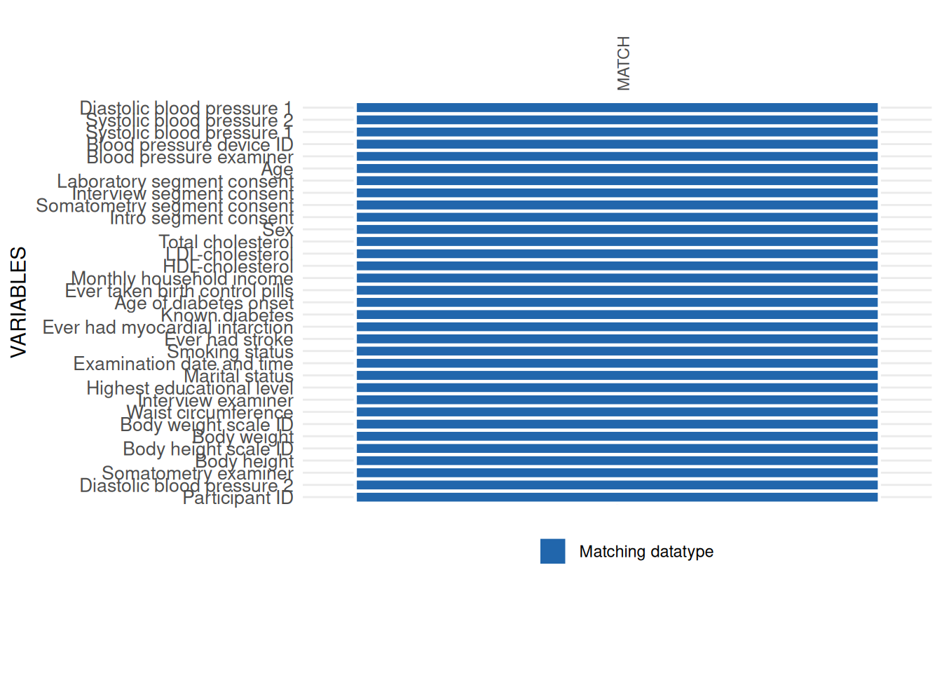
Completeness
The next major step in the data quality assessment workflow is to assess the occurrence and patterns of missing data. The sequence of checks in this example is ordered according to common stages of data collection:
| Level | Description |
|---|---|
| Unit missingness | Subjects without information on any of the provided study variables |
| Segment missingness | Subjects without information for all variables on a defined study segment (e.g., some examination) |
| Item missingness | Subjects without information on data fields within segments |
Following this sequence enables calculating the correct denominators to compute item missingness. Such calculations are particularly important for complex cohort studies in which different levels of examination programs are conducted. For example, only half of a study population might be selected for an MRI examination. In the remaining 50%, the respective MRI variables are not included per study design. This design should be considered if item missingness is examined. For segment missingness, please see the respective tutorial.
Missing values
This check identifies subjects without any measurements on the provided target variables, that is crude missingness.
Note: The interpretation of findings depends on the scope of the provided variables and data records. In this example, the study data set comprises examined SHIP participants, not the target sample. Accordingly, the check is not about study participation. Rather, it identifies cases for which (unexpectedly) no information has been provided. Any identified case would indicate a data management problem.
Missing values can be assessed
with (com_unit_missingness):
my_unit_missings2 <- com_unit_missingness(
  study_data  = sd1,
  meta_data   = meta_data_item,
  label_col   = "LABEL",
  id_vars     = "ID"
)my_unit_missings2$SummaryData| N | X. |
|---|---|
| 0 | 0 |
In total 0 units have missings in all variables of the study data. Thus, for each participant there is at least one variable with information.
Uncertain missingness status, missing due to specified reason, and missing values
The final check in the Completeness dimension identifies
subjects with missing information in variables of all study segments. Uncertain missingness status, Missing due to specified reason, and Missing values can be assessed using com_item_missingness
as in the following call:
item_miss <- com_item_missingness(
  study_data      = sd1,
  meta_data       = meta_data_item,
  show_causes     = TRUE,
  label_col       = "LABEL",
  include_sysmiss = TRUE,
  threshold_value = 95
)
A result overview can be obtained by requesting a summary table of this function:
item_miss$SummaryTable| Variables | Expected observations N | Sysmiss N | Datavalues N | Missing codes N | Jumps N | Measurements N | Missing_expected_obs | PCT_com_crm_mv | GRADING |
|---|---|---|---|---|---|---|---|---|---|
| ID | 2154 | 0 | 2154 | 0 | 0 | 2154 | 0 | 0.00 | 0 |
| EXAM_DT_0 | 2154 | 0 | 2154 | 0 | 0 | 2154 | 0 | 0.00 | 0 |
| SEX_0 | 2154 | 0 | 2154 | 0 | 0 | 2154 | 0 | 0.00 | 0 |
| AGE_0 | 2154 | 0 | 2154 | 0 | 0 | 2154 | 0 | 0.00 | 0 |
| OBS_BP_0 | 2154 | 0 | 2154 | 3 | 0 | 2151 | 3 | 0.14 | 0 |
| DEV_BP_0 | 2154 | 0 | 2154 | 3 | 0 | 2151 | 3 | 0.14 | 0 |
| SBP_0.1 | 2154 | 2 | 2152 | 0 | 0 | 2152 | 2 | 0.09 | 0 |
| SBP_0.2 | 2154 | 6 | 2148 | 0 | 0 | 2148 | 6 | 0.28 | 0 |
| DBP_0.1 | 2154 | 2 | 2152 | 0 | 0 | 2152 | 2 | 0.09 | 0 |
| DBP_0.2 | 2154 | 6 | 2148 | 0 | 0 | 2148 | 6 | 0.28 | 0 |
| OBS_SOMA_0 | 2154 | 0 | 2154 | 2 | 0 | 2152 | 2 | 0.09 | 0 |
| BODY_HEIGHT_0 | 2154 | 3 | 2151 | 0 | 0 | 2151 | 3 | 0.14 | 0 |
| DEV_HEIGHT_0 | 2154 | 0 | 2154 | 2 | 0 | 2152 | 2 | 0.09 | 0 |
| BODY_WEIGHT_0 | 2154 | 4 | 2150 | 0 | 0 | 2150 | 4 | 0.19 | 0 |
| DEV_WEIGHT_0 | 2154 | 0 | 2154 | 2 | 0 | 2152 | 2 | 0.09 | 0 |
| WAIST_CIRC_0 | 2154 | 3 | 2151 | 0 | 0 | 2151 | 3 | 0.14 | 0 |
| OBS_INT_0 | 2154 | 0 | 2154 | 1 | 0 | 2153 | 1 | 0.05 | 0 |
| SCHOOL_GRAD_0 | 2154 | 0 | 2154 | 113 | 0 | 2041 | 113 | 5.25 | 1 |
| RELATION_STATUS_0 | 2154 | 0 | 2154 | 67 | 0 | 2087 | 67 | 3.11 | 0 |
| SMOKING_STATUS_0 | 2154 | 0 | 2154 | 68 | 0 | 2086 | 68 | 3.16 | 0 |
| STROKE_YN_0 | 2154 | 0 | 2154 | 70 | 0 | 2084 | 70 | 3.25 | 0 |
| MYOCARD_YN_0 | 2154 | 0 | 2154 | 74 | 0 | 2080 | 74 | 3.44 | 0 |
| DIABETES_KNOWN_0 | 2154 | 0 | 2154 | 7 | 0 | 2147 | 7 | 0.32 | 0 |
| DIAB_AGE_ONSET_0 | 2154 | 0 | 2154 | 7 | 1974 | 173 | 1981 | 91.97 | 0 |
| CONTRACEPTIVA_EVER_0 | 2154 | 0 | 2154 | 4 | 1264 | 886 | 1268 | 58.87 | 0 |
| HOUSE_INCOME_MONTH_0 | 2154 | 0 | 2154 | 116 | 0 | 2038 | 116 | 5.39 | 1 |
| CHOLES_HDL_0 | 2154 | 16 | 2138 | 0 | 0 | 2138 | 16 | 0.74 | 0 |
| CHOLES_LDL_0 | 2154 | 28 | 2126 | 0 | 0 | 2126 | 28 | 1.30 | 0 |
| CHOLES_ALL_0 | 2154 | 15 | 2139 | 0 | 0 | 2139 | 15 | 0.70 | 0 |
| SEG_PART_INTRO | 2154 | 0 | 2154 | 2154 | 0 | 0 | 2154 | 100.00 | 1 |
| SEG_PART_SOMATOMETRY | 2154 | 0 | 2154 | 2154 | 0 | 0 | 2154 | 100.00 | 1 |
| SEG_PART_INTERVIEW | 2154 | 0 | 2154 | 2154 | 0 | 0 | 2154 | 100.00 | 1 |
| SEG_PART_LABORATORY | 2154 | 0 | 2154 | 2154 | 0 | 0 | 2154 | 100.00 | 1 |
The table provides one line for each of the 29 variables. Of particular interest are:
- System missings (Sysmiss): the number and percentage of data fields for each variable without any valid data entry, indicating a non-informative missing value (Uncertain missingness status).
- Missing Codes: the number and percentage of data fields with valid missing codes.
- Jumps: the number and percentage of data fields for which no data collection was attempted.
- Measurements: provides an inverse of Missing values.
The table shows that the variable HOUSE_INCOME_MONTH_0
(monthly net household income) is affected by many missing values. In
addition, the age of diabetes onset (DIAB_AGE_ONSET_0) was
only coded for 173 subjects, but most values are missing because of an
intended jump.
Note: In case jump codes have been used, e.g., for
the variable CONTRACEPTIVE_EVER_0, the denominator for
calculating item missingness is corrected for the number of jump codes
used.
The summary plot delivers a different view of missing data by providing the frequency of the specified reasons for missing data.
p <- print(item_miss$ReportSummaryTable, view = FALSE)
p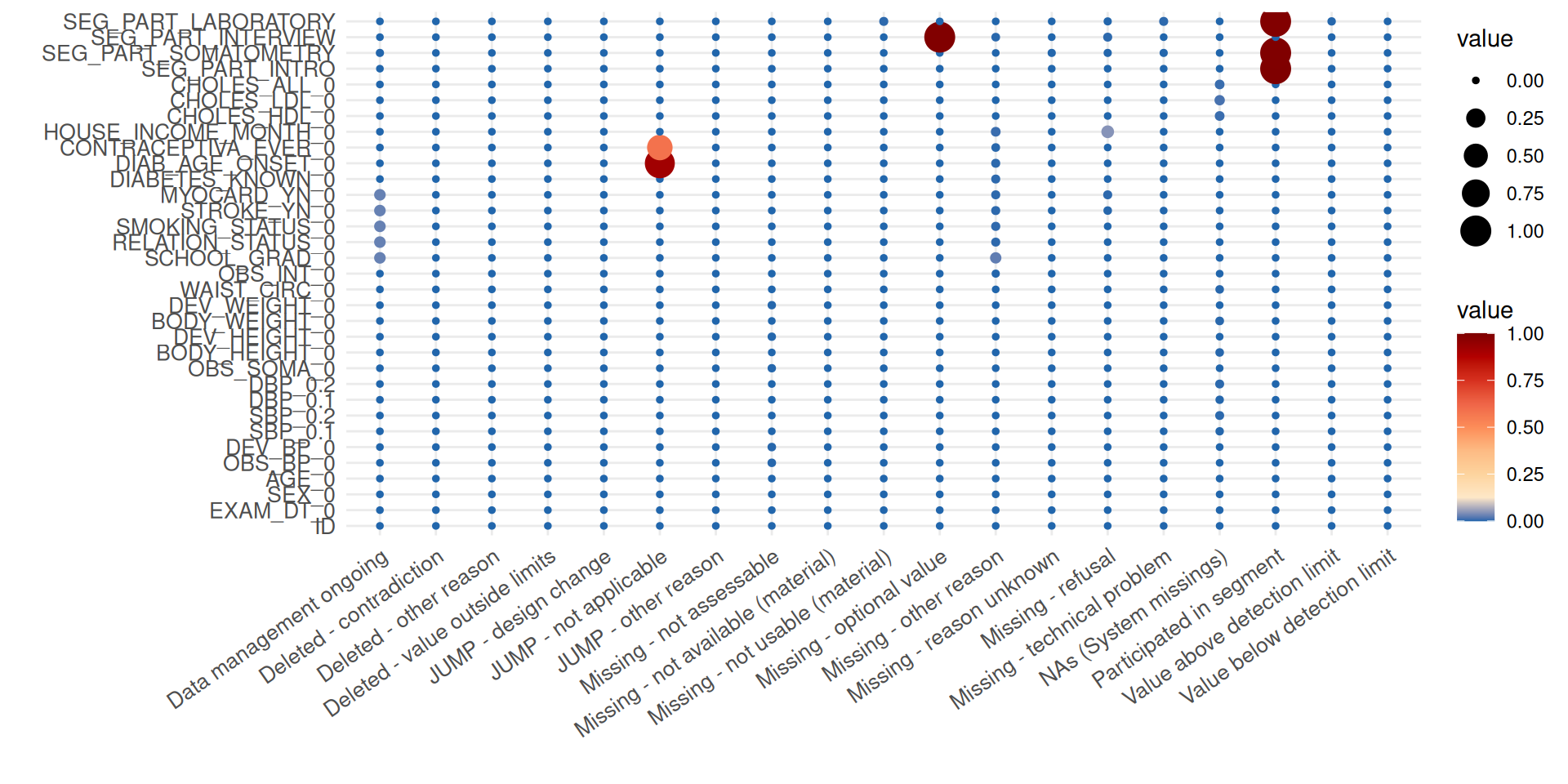
In the plot, the balloon size is determined by the number of missing
data fields. It can now be inferred that, for example, the elevated
number of missing values for the item HOUSE_INCOME_MONTH_0
is mainly caused by refusals of participants to answer the respective
question.
Consistency
Consistency is targeted after completeness has been examined because it requires data without missing and jump codes. Consistency (a main aspect of correctness), describes the degree to which data values are free of breaks in conventions or contradictions. Different data types may be addressed in respective checks.
Uncertain numerical values and Inadmissible numerical values
Both Uncertain numerical values
and Inadmissible numerical values can
be calculated using con_limit_deviations).
When specifying limits = "SOFT_LIMITS" the check does not
identify inadmissible but uncertain values, according to the specified
ranges. An example call is:
MyValueLimits <- con_limit_deviations(
study_data = sd1,
meta_data = meta_data_item,
label_col = "LABEL",
limits = "HARD_LIMITS"
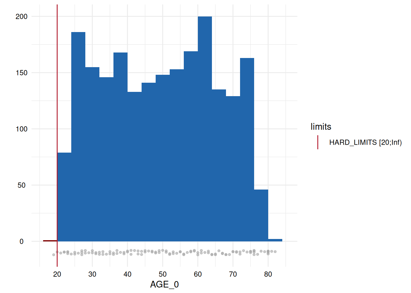
)A table output provides the number and percentage of all the range violations for the variables specifying limits in the metadata:
MyValueLimits$SummaryData| Variables | Limits | Below limits N (%) | Within limits N (%) | Above limits N (%) | All outside limits N (%) | |
|---|---|---|---|---|---|---|
| 1 | DBP_0.2 | HARD_LIMITS | 0 (0) | 2148 (100) | 0 (0) | 0 (0) |
| 5 | DBP_0.2 | DETECTION_LIMITS | 0 (0) | 2148 (100) | 0 (0) | 0 (0) |
| 9 | DBP_0.2 | SOFT_LIMITS | 4 (0.19) | 2134 (99.35) | 10 (0.47) | 14 (0.65) |
| 13 | BODY_HEIGHT_0 | HARD_LIMITS | 0 (0) | 2151 (100) | 0 (0) | 0 (0) |
| 17 | BODY_WEIGHT_0 | HARD_LIMITS | 0 (0) | 2150 (100) | 0 (0) | 0 (0) |
| 21 | WAIST_CIRC_0 | HARD_LIMITS | 0 (0) | 2151 (100) | 0 (0) | 0 (0) |
| 25 | EXAM_DT_0 | HARD_LIMITS | 0 (0) | 2154 (100) | 0 (0) | 0 (0) |
| 29 | CHOLES_HDL_0 | HARD_LIMITS | 0 (0) | 2138 (100) | 0 (0) | 0 (0) |
| 33 | CHOLES_LDL_0 | HARD_LIMITS | 0 (0) | 2126 (100) | 0 (0) | 0 (0) |
| 37 | CHOLES_ALL_0 | HARD_LIMITS | 0 (0) | 2139 (100) | 0 (0) | 0 (0) |
| 41 | AGE_0 | HARD_LIMITS | 1 (0.05) | 2153 (99.95) | 0 (0) | 1 (0.05) |
| 45 | SBP_0.1 | HARD_LIMITS | 0 (0) | 2131 (99.02) | 21 (0.98) | 21 (0.98) |
| 49 | SBP_0.1 | DETECTION_LIMITS | 0 (0) | 2131 (100) | 0 (0) | 0 (0) |
| 53 | SBP_0.1 | SOFT_LIMITS | 4 (0.19) | 2031 (95.31) | 96 (4.5) | 100 (4.69) |
| 57 | SBP_0.2 | HARD_LIMITS | 0 (0) | 2134 (99.35) | 14 (0.65) | 14 (0.65) |
| 61 | SBP_0.2 | DETECTION_LIMITS | 0 (0) | 2134 (100) | 0 (0) | 0 (0) |
| 65 | SBP_0.2 | SOFT_LIMITS | 4 (0.19) | 2071 (97.05) | 59 (2.76) | 63 (2.95) |
| 69 | DBP_0.1 | HARD_LIMITS | 0 (0) | 2150 (99.91) | 2 (0.09) | 2 (0.09) |
| 73 | DBP_0.1 | DETECTION_LIMITS | 0 (0) | 2150 (100) | 0 (0) | 0 (0) |
| 77 | DBP_0.1 | SOFT_LIMITS | 2 (0.09) | 2139 (99.49) | 9 (0.42) | 11 (0.51) |
The last column of the table also provides a GRADING. If the
percentage of violations is above some threshold, a GRADING of 1 is
assigned. In this case, any occurrence is classified as problematic.
Otherwise, the GRADING is 0.
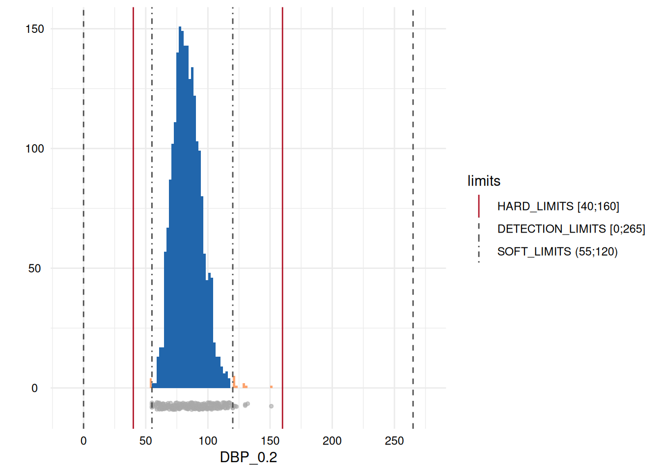
The following statement assigns all variables identified as
problematic to an object whichdeviate to enable a more
targeted output, for example, to plot the distributions for any variable
with violations along the specified limits:
# select variables with deviations
whichdeviate <- as.character(
  MyValueLimits$SummaryTable$Variables)[
    MyValueLimits$SummaryTable$FLG_con_rvv_unum == 1 |
    MyValueLimits$SummaryTable$FLG_con_rvv_utdat == 1 |
    MyValueLimits$SummaryTable$FLG_con_rvv_inum == 1 |
    MyValueLimits$SummaryTable$FLG_con_rvv_itdat == 1                    ]
whichdeviate <- whichdeviate[!is.na(whichdeviate)]
We can restrict the plots to those where variables have limit
deviations, i.e., those with a GRADING of 1 in the table above, using
MyValueLimits$SummaryPlotList[whichdeviate] (only the first
two are displayed below to reduce file size):
Inadmissible categorical values
A comparable check may be performed for Inadmissible categorical values using con_inadmissible_categorical):
IAVCatAll <- con_inadmissible_categorical(
  study_data = sd1,
  meta_data  = meta_data_item,
  label_col  = "LABEL"
)
As with inadmissible numerical values, a table output displays the observed categories, the defined categories, any non matching level, its count, and a GRADING:
IAVCatAll$SummaryData| Variables | OBSERVED_CATEGORIES | DEFINED_CATEGORIES | NON_MATCHING | NON_MATCHING_N | NON_MATCHING_N_PER_CATEGORY |
|---|---|---|---|---|---|
| OBS_SOMA_0 | 1, 2, 3, 4, 5, 7, 8, 9 | 1, 2, 3, 4, 5, 6, 7, 8, 9, 10 | 0 | 0 | |
| DEV_HEIGHT_0 | 3, 4, 11 | 1, 2, 3, 4, 5, 6, 7, 8, 9, 10, 11, 12, 13, 14, 15, 16, 17, 18, 19, 20, 21, 22, 23, 24, 25 | 0 | 0 | |
| DEV_WEIGHT_0 | 1, 2, 11 | 1, 2, 3, 4, 5, 6, 7, 8, 9, 10, 11, 12, 13, 14, 15, 16, 17, 18, 19, 20, 21, 22, 23, 24, 25 | 0 | 0 | |
| OBS_INT_0 | 1, 2, 3, 4, 5, 7, 10, 11, 12, 13, 22, 23, 25 | 1, 2, 3, 4, 5, 6, 7, 8, 9, 10, 11, 12, 13, 14, 15, 16, 17, 18, 19, 20, 21, 22, 23, 24, 25 | 0 | 0 | |
| SCHOOL_GRAD_0 | 0, 1, 2, 3, 4 | 0, 1, 2, 3 | 4 | 7 | 7 (“4”) |
| RELATION_STATUS_0 | 1, 2, 3, 4, 5 | 1, 2, 3, 4, 5 | 0 | 0 | |
| SMOKING_STATUS_0 | 0, 1, 2 | 0, 1, 2 | 0 | 0 | |
| STROKE_YN_0 | 1, 2 | 1, 2 | 0 | 0 | |
| MYOCARD_YN_0 | 1, 2 | 1, 2 | 0 | 0 | |
| DIABETES_KNOWN_0 | 0, 1 | 0, 1 | 0 | 0 | |
| CONTRACEPTIVA_EVER_0 | 1, 2 | 1, 2 | 0 | 0 | |
| HOUSE_INCOME_MONTH_0 | 1, 2, 3 | 1, 2, 3 | 0 | 0 | |
| SEX_0 | 1, 2 | 1, 2 | 0 | 0 | |
| OBS_BP_0 | 1, 3, 4, 5, 7, 8, 9, 11, 16, 18 | 1, 2, 3, 4, 5, 6, 7, 8, 9, 10, 11, 12, 13, 14, 15, 16, 17, 18, 19, 20 | 0 | 0 | |
| DEV_BP_0 | 7, 9, 10, 14, 15, 16, 17, 18, 19, 20, 22 | 1, 2, 3, 4, 5, 6, 7, 8, 9, 10, 11, 12, 13, 14, 15, 16, 17, 18, 19, 20, 21, 22, 23, 24, 25 | 0 | 0 |
The results show that there is one variable, SCHOOL_GRAD_0, with one inadmissible level occurring.
Accuracy
In contrast to most consistency related indicators, accuracy findings indicate an elevated probability that some data quality issue exists, rather than a certain issue.
Univariate outliers
Univariate outliers are assessed
based on statistical criteria. The function acc_robust_univariate_outlier
identifies outliers according to the approaches of Tukey,
3SD, Hubert,
and the heuristic approach of SigmaGap. It may be called as
follows:
UnivariateOutlier <- acc_robust_univariate_outlier(
  study_data = sd1,
  meta_data = meta_data_item,
  label_col = "LABEL"
)
The first output is a table that provides descriptive statistics and detected outliers according to the different criteria:
UnivariateOutlier$SummaryTable| Variables | Mean | No.records | SD | Median | Skewness | Tukey (N) | 3SD (N) | Hubert (N) | Sigma-gap (N) | NUM_acc_ud_outlu | Outliers, low (N) | Outliers, high (N) | GRADING | PCT_acc_ud_outlu |
|---|---|---|---|---|---|---|---|---|---|---|---|---|---|---|
| ID | 5431.06 | 2154 | 1236.17 | 5428.50 | 0.00 | 0 | 0 | 0 | 0 | 0 | 0 | 0 | 0 | 0.00 |
| DBP_0.2 | 83.52 | 2148 | 11.52 | 83.00 | 0.04 | 17 | 10 | 10 | 1 | 1 | 0 | 1 | 1 | 0.05 |
| BODY_HEIGHT_0 | 168.22 | 2151 | 9.25 | 168.00 | 0.00 | 1 | 1 | 1 | 0 | 0 | 0 | 0 | 0 | 0.00 |
| BODY_WEIGHT_0 | 77.63 | 2150 | 15.08 | 77.04 | 0.01 | 17 | 10 | 15 | 0 | 0 | 0 | 0 | 0 | 0.00 |
| WAIST_CIRC_0 | 89.20 | 2151 | 13.82 | 89.52 | -0.05 | 6 | 6 | 15 | 0 | 0 | 0 | 0 | 0 | 0.00 |
| DIAB_AGE_ONSET_0 | 53.68 | 173 | 13.33 | 55.00 | 0.00 | 5 | 3 | 5 | 0 | 0 | 0 | 0 | 0 | 0.00 |
| CHOLES_HDL_0 | 1.45 | 2138 | 0.44 | 1.39 | 0.13 | 33 | 17 | 18 | 2 | 2 | 0 | 2 | 1 | 0.09 |
| CHOLES_LDL_0 | 3.58 | 2126 | 1.13 | 3.52 | 0.02 | 21 | 13 | 18 | 0 | 0 | 0 | 0 | 0 | 0.00 |
| CHOLES_ALL_0 | 5.76 | 2139 | 1.20 | 5.68 | 0.06 | 23 | 12 | 17 | 0 | 0 | 0 | 0 | 0 | 0.00 |
| AGE_0 | 49.87 | 2153 | 16.18 | 50.00 | -0.02 | 0 | 0 | 0 | 0 | 0 | 0 | 0 | 0 | 0.00 |
| SBP_0.1 | 138.25 | 2131 | 21.25 | 137.00 | 0.06 | 8 | 0 | 4 | 0 | 0 | 0 | 0 | 0 | 0.00 |
| SBP_0.2 | 135.87 | 2134 | 20.89 | 134.00 | 0.09 | 10 | 5 | 3 | 0 | 0 | 0 | 0 | 0 | 0.00 |
| DBP_0.1 | 84.43 | 2150 | 11.43 | 84.00 | 0.00 | 17 | 12 | 15 | 1 | 1 | 0 | 1 | 1 | 0.05 |
There are outliers according to at least two criteria in most variables, but only for the diastolic blood pressure variables (DBP_0.1 and DBP_0.2) two outliers have been detected using the Sigma-gap criterion.
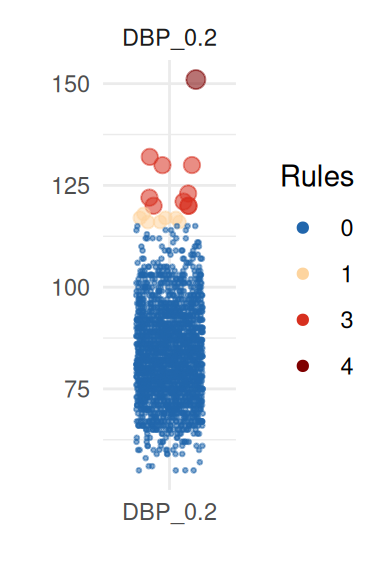
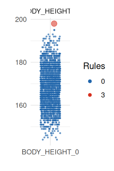
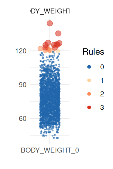
To obtain a better insight on univariate distributions, a plot is
provided (call it with UnivariateOutlier$SummaryPlotList).
It highlights observations for each variable according to the number of
violated rules (only the first four are shown here):
pl <- UnivariateOutlier$SummaryPlotList

invisible(lapply(head(pl, 4), print))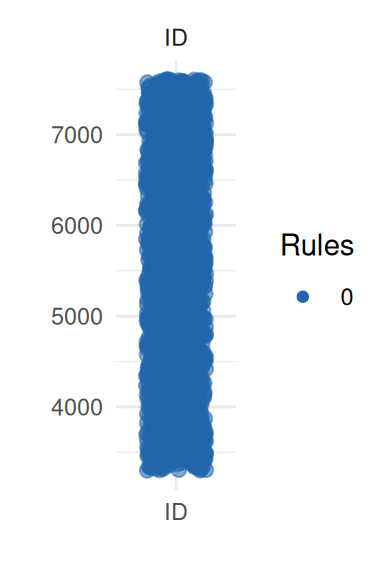
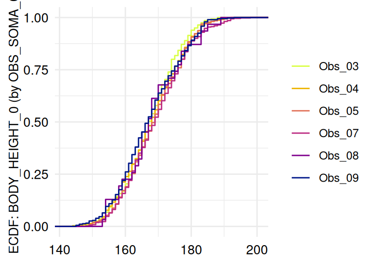
Unexpected location and proportion
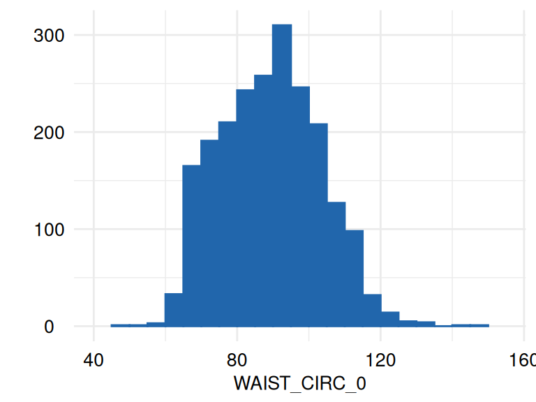
The function acc_distributions
examines Unexpected location and Unexpected proportion using histograms
and displays empirical cumulative distribution functions (ecdf) if a
grouping variable is provided.
The following example examines measurements in which a possible influence of the examiners is considered:
ECDFSoma1 <- acc_distributions(
study_data = sd1,
meta_data = meta_data_item,
resp_vars = c("WAIST_CIRC_0", "BODY_HEIGHT_0", "BODY_WEIGHT_0"),
label_col = "LABEL"
)
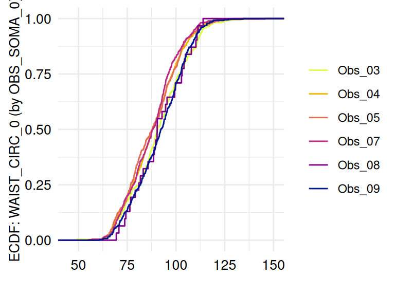
ECDFSoma2 <- acc_distributions_ecdf(
study_data = sd1,
meta_data = meta_data_item,
resp_vars = c("WAIST_CIRC_0", "BODY_HEIGHT_0", "BODY_WEIGHT_0"),
group_vars = "OBS_SOMA_0",
label_col = "LABEL"
)The respective list of plots may be displayed using
ECDFSoma$SummaryPlotList (only the first 2 plots are
displayed below):
The function acc_margins is also
related to these indicators. However, it also provides descriptive
outputs, such as violin and box plots for continuous variables, count
plots for categorical data, and density plots for both. The main
application of acc_margins is to make
inference on effects related to process variables, such as examiners,
devices, or study centers. The function determines whether measurements
are continuous or discrete. Alternatively, this information may be
specified in the metadata.
In the example, acc_margins is applied
to the variable waist circumference (WAIST_CIRC_0). In this
case, dependencies related to the examiners (OBS_SOMA_0) are
assessed, while the raw measurements are controlled for variable age and
sex (AGE_0, SEX_0):
marginal_dists <- acc_margins(
  study_data      = sd1,
  meta_data       = meta_data_item,
  resp_vars  = "WAIST_CIRC_0",
  co_vars    = c("AGE_0", "SEX_0"),
  group_vars = "OBS_SOMA_0",
  label_col  = "LABEL"
)
A plot is provided to view the results:
marginal_dists$SummaryPlot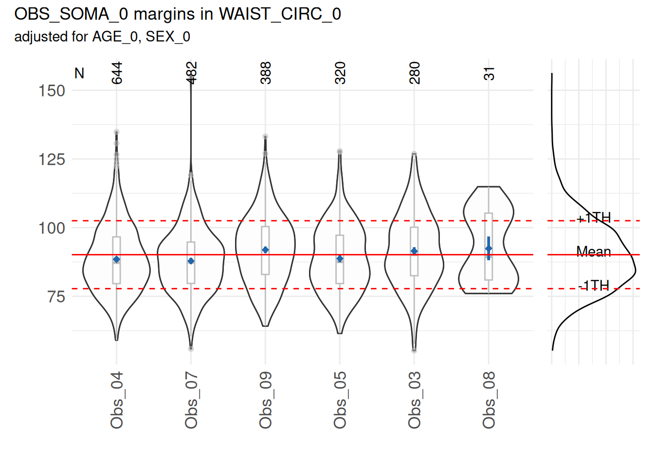
Based on a statistical test, no mean waist circumference of any examiner differed substantially (p<0.05) from the overall mean.
However, some examiners can have a mean that differ from the overall mean. This can be observed in the following example, where the measurements of waist circumference of the examiner “3” have been increased by 20.
#increase by 20 the measurements of observer 3
sd1_example <- dplyr::mutate(sd1, waist= ifelse(obs_soma == "3", waist+20, waist))

marginal_dists <- acc_margins(
    study_data      = sd1_example ,
    meta_data       = meta_data_item,
    resp_vars  = "WAIST_CIRC_0",
    co_vars    = c("AGE_0", "SEX_0"),
    group_vars = "OBS_SOMA_0",
    label_col  = "LABEL"
)

marginal_dists$SummaryPlot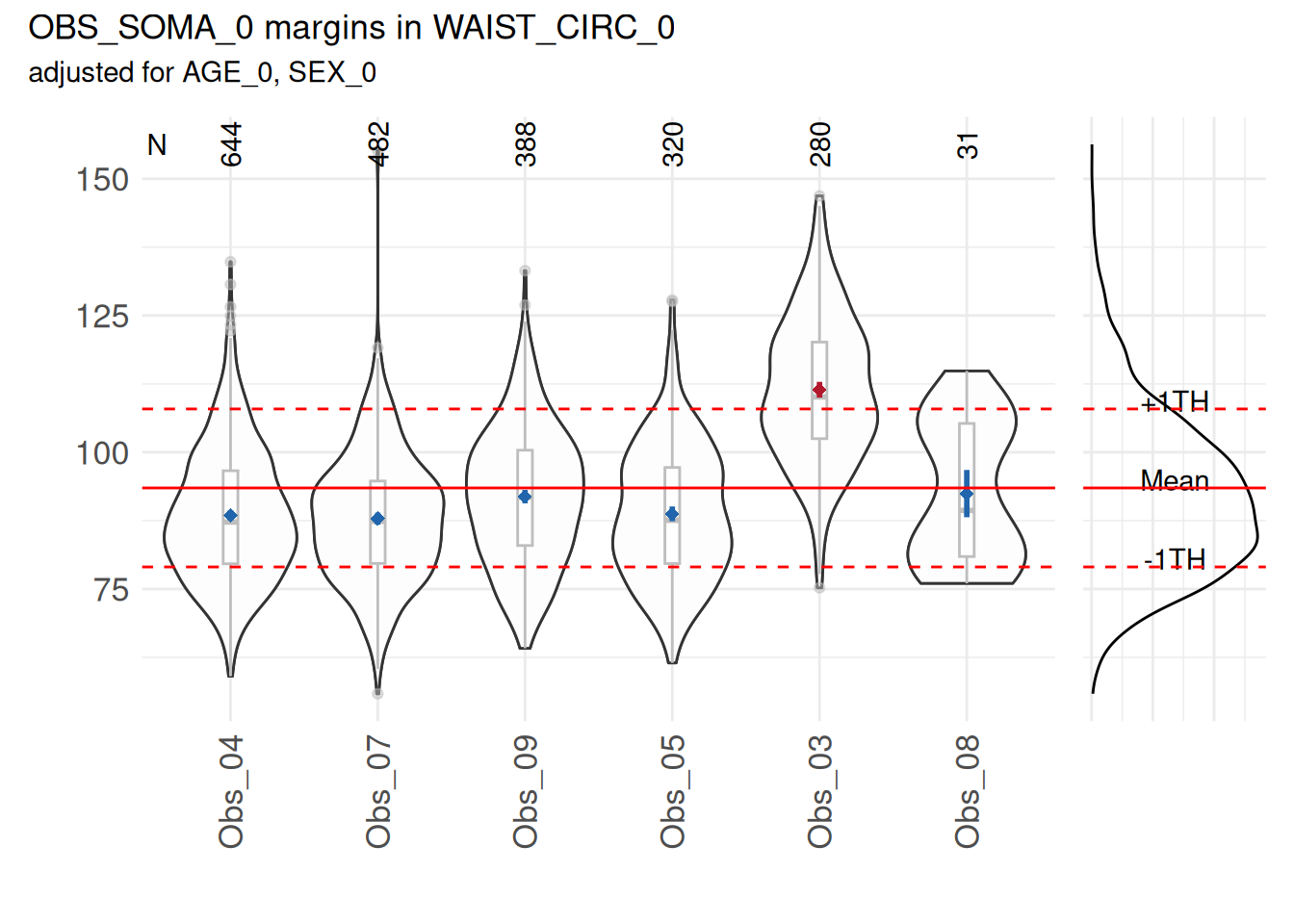
The result shows elevated proportions for the examiner 03.
Variance components
An important and related issue is the quantification of the observed
examiner effects, which is accomplished by the function acc_varcomp. acc_varcomp computes
the percentage of variance for some target variable, here attributable
to the grouping variable while controlling for some other variables (age
and sex). The output may be reviewed in a table format:
vcs_waist <- acc_varcomp(
  study_data = sd1,
  meta_data  = meta_data_item,
  resp_vars  = "WAIST_CIRC_0",
  co_vars    = c("AGE_0", "SEX_0"),
  group_vars = "OBS_SOMA_0",
  label_col  = "LABEL"
)vcs_waist$SummaryTable| Variables | Object | Model.Call | ICC_acc_ud_loc | Class.Number | Mean.Class.Size | Median.Class.Size | Min.Class.Size | Max.Class.Size | convergence.problem |
|---|---|---|---|---|---|---|---|---|---|
| WAIST_CIRC_0 | OBS_SOMA_0 | WAIST_CIRC_0 ~ AGE_0 + SEX_0 + (1 | OBS_SOMA_0) | 0.019 | 6 | 357.5 | 354 | 31 | 644 | FALSE |
For the variable WAIST_CIRC_0, an ICC of 0.019 has been found which is below the threshold. The same is the case for the variable CHOLES_HDL_0:
vcs_chol <- acc_varcomp(
  study_data = sd1,
  meta_data = meta_data_item,
  resp_vars = "CHOLES_HDL_0",
  co_vars =c("AGE_0", "SEX_0"),
  group_vars = "OBS_INT_0",
  label_col = "LABEL"
)vcs_chol$SummaryTable| Variables | Object | Model.Call | ICC_acc_ud_loc | Class.Number | Mean.Class.Size | Median.Class.Size | Min.Class.Size | Max.Class.Size | convergence.problem |
|---|---|---|---|---|---|---|---|---|---|
| CHOLES_HDL_0 | OBS_INT_0 | CHOLES_HDL_0 ~ AGE_0 + SEX_0 + (1 | OBS_INT_0) | 0.024 | 10 | 213 | 178 | 10 | 596 | FALSE |
LOESS
The study of effects across groups and times is particularly complex.
The function acc_loess provides a
descriptor related to the indicator Unexpected location. acc_loess may also be
used to obtain information related to other indicators in the domain of
unexpected distributions.
An example call using waist circumference as the target variable is:
timetrends <- acc_loess(
  study_data = sd1,
  meta_data  = meta_data_item,
  resp_vars  = "WAIST_CIRC_0",
  co_vars    = c("AGE_0", "SEX_0"),
  group_vars = "OBS_SOMA_0",
  time_vars  = "EXAM_DT_0",
  label_col  = "LABEL"
)

invisible(lapply(timetrends$SummaryPlotList, print))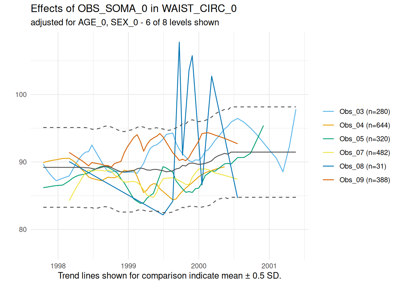
The graph for this variable indicates no major discrepancies between the examiners over the examination period.
Unexpected scale and shape
Assessing the shape of a distribution is, next to location
parameters, an important aspect of accuracy. Observed distributions can
be tested against expected distributions using the function acc_shape_or_scale.
In this example the normal distribution of blood pressure is
examined:
MyUnexpDist2 <- acc_shape_or_scale(
  study_data = sd1,
  meta_data  = meta_data_item,
  resp_vars  = "SBP_0.2",
  guess      = TRUE,
  label_col  =  "LABEL",
  dist_col   = "DISTRIBUTION",
)

MyUnexpDist2$SummaryPlot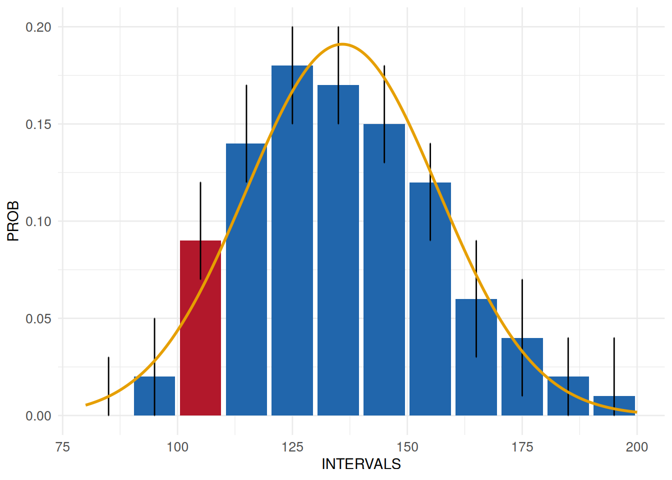
The result reveals a slight discrepancy from the normality assumption. It is up to the person responsible for the data quality assessments to decide whether such a discrepancy is relevant.
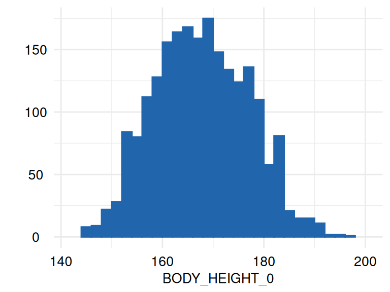
The analysis of end digit preferences is a specific implementation of
Unexpected shape. In this example,
the uniform distribution of the end digits of body height are examined
using acc_end_digits.
Body height in SHIP-START-0 was a measurement which required the manual
reading and transfer of data into an eCRF.
MyEndDigits <- acc_end_digits(
  study_data = sd1,
  meta_data  = meta_data_item,
  resp_vars  = "BODY_HEIGHT_0",
  label_col  = "LABEL"
)

MyEndDigits$SummaryPlot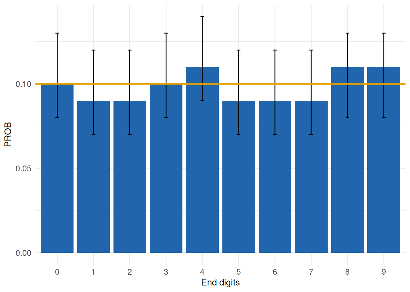
The graph highlights no relevant effects across the ten categories. Output within the accuracy dimension frequently combines descriptive and inferential content, which is necessary to facilitate valid conclusions on data quality issues. Further details on all functions can be obtained following the links and in the Software section.
